Analysis of the Searhose data of DLBCL cell lines
Junyan Lu
Last updated: 2024-05-27
Checks: 5 1
Knit directory: combiDLBCL/analysis/
This reproducible R Markdown analysis was created with workflowr (version 1.7.0). The Checks tab describes the reproducibility checks that were applied when the results were created. The Past versions tab lists the development history.
Great job! The global environment was empty. Objects defined in the global environment can affect the analysis in your R Markdown file in unknown ways. For reproduciblity it’s best to always run the code in an empty environment.
The command set.seed(20220425) was run prior to running
the code in the R Markdown file. Setting a seed ensures that any results
that rely on randomness, e.g. subsampling or permutations, are
reproducible.
Great job! Recording the operating system, R version, and package versions is critical for reproducibility.
Nice! There were no cached chunks for this analysis, so you can be confident that you successfully produced the results during this run.
Great job! Using relative paths to the files within your workflowr project makes it easier to run your code on other machines.
Tracking code development and connecting the code version to the
results is critical for reproducibility. To start using Git, open the
Terminal and type git init in your project directory.
This project is not being versioned with Git. To obtain the full
reproducibility benefits of using workflowr, please see
?wflow_start.
Load libraries
Read Seahorse data table
Read excel file
rawPath <- "../data/Terzidou/Seahorse/"
allFiles <- list.files(rawPath, pattern = "SH_.*xlsx", recursive = TRUE)
seaTabRaw <- lapply(allFiles, function(fileName) {
  plateName <- str_extract(fileName, "SH_[0-9]+")
  eachTab <- readxl::read_xlsx(paste0(rawPath, fileName), sheet = 5) %>%
    mutate(plate = plateName)
}) %>% bind_rows() %>%
  mutate(Drug = str_extract(Group, "DMSO|MI-2|Control|(MALT1 inhibitor)"),
         cellLine = str_extract(Group, "OCI-LY3|U-2940|HBL-1|WSU-DLCL-2|Balm-3|TMD-8|SC-1|U-2932|K-422")) %>%
  filter(Group != "Background") %>%
  pivot_longer(c(OCR,ECAR,PER), names_to = "measure", values_to = "value") %>%
  dplyr::rename(timeStep = Measurement)
Check experimental design
table(seaTabRaw$cellLine, seaTabRaw$Drug,seaTabRaw$plate ), , = SH_401
Control DMSO MALT1 inhibitor MI-2
Balm-3 0 0 0 0
HBL-1 0 0 0 0
K-422 0 0 0 0
OCI-LY3 363 396 363 396
SC-1 0 0 0 0
TMD-8 0 0 0 0
U-2932 0 0 0 0
U-2940 363 396 363 396
WSU-DLCL-2 0 0 0 0
, , = SH_402
Control DMSO MALT1 inhibitor MI-2
Balm-3 0 0 0 0
HBL-1 0 264 231 264
K-422 0 0 0 0
OCI-LY3 0 231 264 264
SC-1 0 0 0 0
TMD-8 0 0 0 0
U-2932 0 0 0 0
U-2940 0 231 264 264
WSU-DLCL-2 0 264 231 264
, , = SH_404
Control DMSO MALT1 inhibitor MI-2
Balm-3 0 231 264 264
HBL-1 0 0 0 0
K-422 0 0 0 0
OCI-LY3 0 0 0 0
SC-1 0 231 264 264
TMD-8 0 264 231 264
U-2932 0 264 231 264
U-2940 0 0 0 0
WSU-DLCL-2 0 0 0 0
, , = SH_406
Control DMSO MALT1 inhibitor MI-2
Balm-3 0 0 0 0
HBL-1 0 0 0 0
K-422 0 528 528 528
OCI-LY3 0 0 0 0
SC-1 0 0 0 0
TMD-8 0 0 0 0
U-2932 0 0 0 0
U-2940 0 0 0 0
WSU-DLCL-2 0 0 0 0
, , = SH_407
Control DMSO MALT1 inhibitor MI-2
Balm-3 0 0 0 0
HBL-1 0 264 264 264
K-422 0 0 0 0
OCI-LY3 0 0 0 0
SC-1 0 0 0 0
TMD-8 0 264 264 264
U-2932 0 198 264 264
U-2940 0 0 0 0
WSU-DLCL-2 0 264 198 264**Some cell lines have 2 biological replicates on two different plates*
Annotate the biological replicates (stored in the rep column)
repTab <- distinct(seaTabRaw, cellLine, plate) %>%
  arrange(cellLine, plate) %>%
  group_by(cellLine) %>% mutate(rep=seq(length(plate))) %>%
  ungroup() %>% mutate(rep = paste0("R",rep))
seaTabRaw <- left_join(seaTabRaw, repTab, by = c("cellLine","plate"))
table(repTab$cellLine, repTab$plate)
             SH_401 SH_402 SH_404 SH_406 SH_407
  Balm-3          0      0      1      0      0
  HBL-1           0      1      0      0      1
  K-422           0      0      0      1      0
  OCI-LY3         1      1      0      0      0
  SC-1            0      0      1      0      0
  TMD-8           0      0      1      0      1
  U-2932          0      0      1      0      1
  U-2940          1      1      0      0      0
  WSU-DLCL-2      0      1      0      0      1
Quality assessment of the raw data
Plot seahorse values along time, per each group
pList <- lapply(unique(seaTabRaw$Group), function(n) {
  plotTab <- filter(seaTabRaw, Group == n) %>% mutate(plateWell = paste0(plate,Well))
  ggplot(plotTab, aes(x=timeStep, y=value, color = plate, plateWell=Well)) +
    geom_point(aes(color = plate)) +
    geom_line() +
    facet_wrap(~measure, ncol=1, scale= "free_y") +
    ggtitle(n)
})
jyluMisc::makepdf(pList, name  = "../docs/seahorseRaw_perGroup.pdf", height = 10, width = 10, figNum = 1, ncol = 1, nrow = 1)
Loading required package: gridExtra
Attaching package: 'gridExtra'The following object is masked from 'package:dplyr':
combinePlot seahorse values along time, per each cell line, to visualze the treatment difference
plotTab <- arrange(seaTabRaw, cellLine, plate) %>%
  mutate(cellLine_plate = paste0(cellLine,"_", plate),
         plateWell = paste0(plate,"_",Well))
pList <- lapply(unique(plotTab$cellLine_plate), function(n) {
  eachTab <- filter(plotTab, cellLine_plate == n)
  ggplot(plotTab, aes(x=timeStep, y=value, color = Drug, group=plateWell)) +
    geom_point(alpha=0.5) +
    geom_line(alpha=0.5) +
    facet_wrap(~measure, ncol=1, scale= "free_y") +
    ggtitle(n)
})
jyluMisc::makepdf(pList, name = "../docs/seahorseRaw_perCellline.pdf", height = 10, width = 10, figNum = 1, ncol = 1, nrow = 1)Deal with outlier wells
Detect outlier well for each plate and time-point using robust z-score
detectOutlier <- function(x, zCut = 3.5) {
  z <- (x-median(x))/mad(x)
  return(abs(z) > zCut)
}
outlierTab <- group_by(seaTabRaw, plate, timeStep, measure) %>%
  mutate(isOutlier = detectOutlier(value, zCut=3.5))
Get the plate and wells that have the most outliers
outlierSum <- group_by(outlierTab, plate, Well) %>% summarise(n = sum(isOutlier)) %>%
  arrange(desc(n))
`summarise()` has grouped output by 'plate'. You can override using the
`.groups` argument.head(outlierSum)# A tibble: 6 × 3
# Groups: plate [3]
plate Well n
<chr> <chr> <int>
1 SH_401 C12 18
2 SH_406 A04 11
3 SH_401 D12 8
4 SH_407 B12 8
5 SH_407 C11 8
6 SH_407 E09 8Remove the wells that counted as outliers for more than three times
removeTab <- filter(outlierSum, n >=3)
seaTabRaw <- left_join(seaTabRaw, removeTab, by = c("plate","Well")) %>%
  filter(is.na(n)) %>%
  select(-n)
Re-do the above searhose plot without outliers
Plot seahorse values along time, per each group
pList <- lapply(unique(seaTabRaw$Group), function(n) {
  plotTab <- filter(seaTabRaw, Group == n) %>% mutate(plateWell = paste0(plate,Well))
  ggplot(plotTab, aes(x=timeStep, y=value, color = plate, plateWell=Well)) +
    geom_point(aes(color = plate)) +
    geom_line() +
    facet_wrap(~measure, ncol=1, scale= "free_y") +
    ggtitle(n)
})
jyluMisc::makepdf(pList, name  = "../docs/seahorseRaw_perGroup_noOutlier.pdf", height = 10, width = 10, figNum = 1, ncol = 1, nrow = 1)
seahorseRaw_perGroup_noOutlier.pdf
The same wells along time are connected by lines
Plot seahorse values along time, per each cell line, to visualze the treatment difference
plotTab <- arrange(seaTabRaw, cellLine, plate) %>%
  mutate(cellLine_plate = paste0(cellLine,"_", plate),
         plateWell = paste0(plate,"_",Well))
pList <- lapply(unique(plotTab$cellLine_plate), function(n) {
  eachTab <- filter(plotTab, cellLine_plate == n)
  ggplot(plotTab, aes(x=timeStep, y=value, color = Drug, group=plateWell)) +
    geom_point(alpha=0.5) +
    geom_line(alpha=0.5) +
    facet_wrap(~measure, ncol=1, scale= "free_y") +
    ggtitle(n)
})
jyluMisc::makepdf(pList, name = "../docs/seahorseRaw_perCellline_noOutlier.pdf", height = 10, width = 10, figNum = 1, ncol = 1, nrow = 1)Summarize metabolic features for each well based on Seahorse formula
CCF = 0.61
seaTab <- mutate(seaTabRaw, stage = case_when(timeStep %in% 1:3 ~ 1,
                                              timeStep %in% 4:6 ~ 2,
                                              timeStep %in% 9:11 ~ 3)) %>%
  filter(!is.na(stage)) %>%
  mutate(measure = paste0(measure,"_",stage)) %>%
  group_by(plate, Well, measure) %>%
  summarise(value = mean(value)) %>%
  pivot_wider(names_from = measure, values_from = value) %>%
  mutate(mitoOCR = OCR_1 - OCR_2,
         mitoPER = mitoOCR*CCF,
         glycoPER = PER_1 - mitoPER) %>%
  dplyr::rename(baseOCR = OCR_1, baseECAR = ECAR_1, comp.glycolysis = PER_2) %>%
  select(plate, Well, glycoPER, baseOCR, baseECAR, comp.glycolysis) %>%
  pivot_longer(-c(plate, Well), names_to = "measure", values_to = "value") %>%
  left_join(distinct(seaTabRaw, Well, Group, plate, Drug, cellLine, rep), by = c("plate","Well"))
`summarise()` has grouped output by 'plate', 'Well'. You can override using the
`.groups` argument.Four values will be derived:
- glycoPER: glycolytic PER, calculated based on the formula from
Seahorse website
- comp.glycolysis: compensatory glycolysis, the PER after adding
Rot/AA
- baseOCR: baseline OCR
- baseECR: baseline ECAR
Visualize the difference among conditions per-cell liens using bar plots
sumTab <- group_by(seaTab, measure, Drug, cellLine, rep) %>%
  summarise(meanVal = mean(value),
            seVal = sd(value)/sqrt(length(Well)-1)) %>%
  mutate(CI = 1.96*seVal) %>% ungroup()
`summarise()` has grouped output by 'measure', 'Drug', 'cellLine'. You can
override using the `.groups` argument.plotTab <- arrange(sumTab, cellLine, rep) %>%
mutate(cellRep = paste0(cellLine,"_",rep))
pList <- lapply(unique(plotTab$cellRep), function(n) {
eachTab <- filter(plotTab, cellRep == n)
dotTab <- filter(seaTab) %>%
mutate(cellRep = paste0(cellLine,"_",rep)) %>%
filter(cellRep == n)
ggplot(eachTab, aes(x=Drug, y = meanVal, fill = Drug)) +
geom_bar(stat="identity") +
ggbeeswarm::geom_quasirandom(data = dotTab, aes(y=value)) +
geom_errorbar(aes(ymax= meanVal+CI, ymin=meanVal-CI), width=0.5, color="darkred") +
facet_wrap(~measure, scale= "free_y") +
ggtitle(n) +
theme(legend.position = "none",
axis.text.x = element_text(angle = 90, hjust = 1, vjust = 0.5)) +
ylab("mean value") + xlab("")
})
cowplot::plot_grid(plotlist = pList, ncol=2)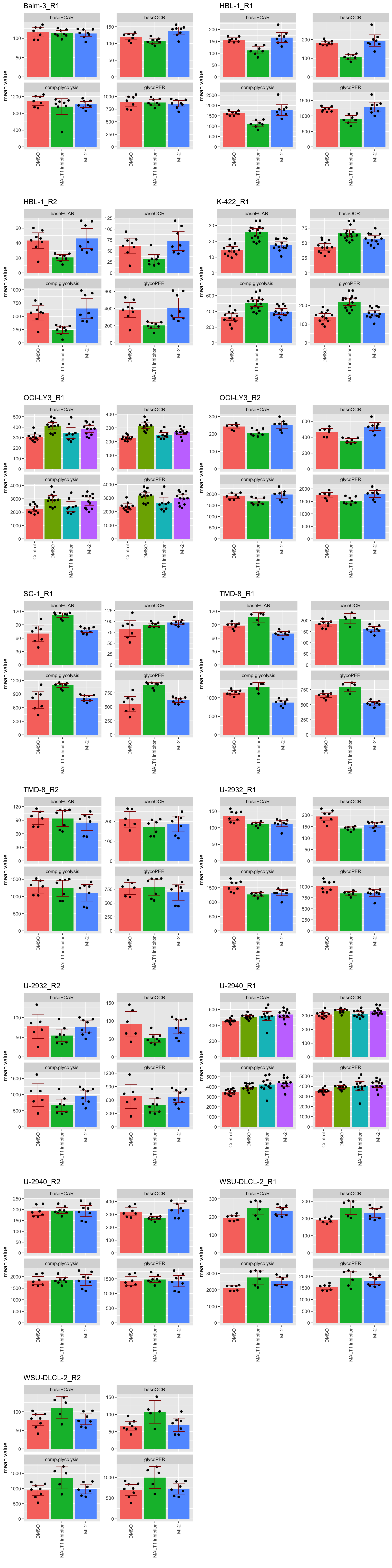
jyluMisc::makepdf(pList, "../docs/seahorse_barplot.pdf", height = 10, width = 10, ncol = 2, nrow=2)Download the pdf file: seahorse_barplot.pdf
The error bars indicate 95% confidence interval. So if the error
bars are not touching, the P-value should be < 0.05
Save the summarised values as a excel table (in a tidy table format)
writexl::write_xlsx(seaTab, "../docs/seahorse_table.xlsx")seahorse_table.xlsx
Note, each well is considered as a technical replicates, which
is shown as the black dot in the bar plot above
Normalize the values by DMSO to allow cross cell line comparison
Normalization (calculate fold change to DMSO)
sumTab <- group_by(seaTab, measure, Drug, cellLine, rep) %>%
  summarise(meanVal = mean(value)) %>% ungroup()
`summarise()` has grouped output by 'measure', 'Drug', 'cellLine'. You can
override using the `.groups` argument.sumTab.drug <- filter(sumTab, !Drug %in% c("DMSO","Control"))
sumTab.dmso <- filter(sumTab, Drug %in% c("DMSO")) %>%
select(-Drug) %>% dplyr::rename(dmsoVal = meanVal)
normTab <- left_join(sumTab.drug, sumTab.dmso, by = c("measure","cellLine","rep")) %>%
mutate(normVal = meanVal/dmsoVal) %>%
mutate(synergyGroup =ifelse(cellLine %in% c("K-422","OCI-LY3","HBL-1","U-2932"),"synergy","non-synergy")) %>%
select(measure, Drug, cellLine, rep, normVal, synergyGroup)Save the DMSO normalized table
writexl::write_xlsx(normTab, "../docs/seahorse_DMSO_normalized.xlsx")Visualization of the normalized values (fold change to DMSO) among synergy and non-synergy cell lines
pList <- lapply(unique(normTab$Drug), function(dd) {
plotTab <- filter(normTab, Drug == dd)
ggplot(plotTab, aes(x=synergyGroup, y=normVal)) +
geom_boxplot() +
geom_point(aes(color = synergyGroup)) +
ggrepel::geom_text_repel(aes(label = cellLine)) +
facet_wrap(~measure, ncol=2) +
ggtitle(dd) +
theme_bw()
})
cowplot::plot_grid(plotlist=pList, ncol=1)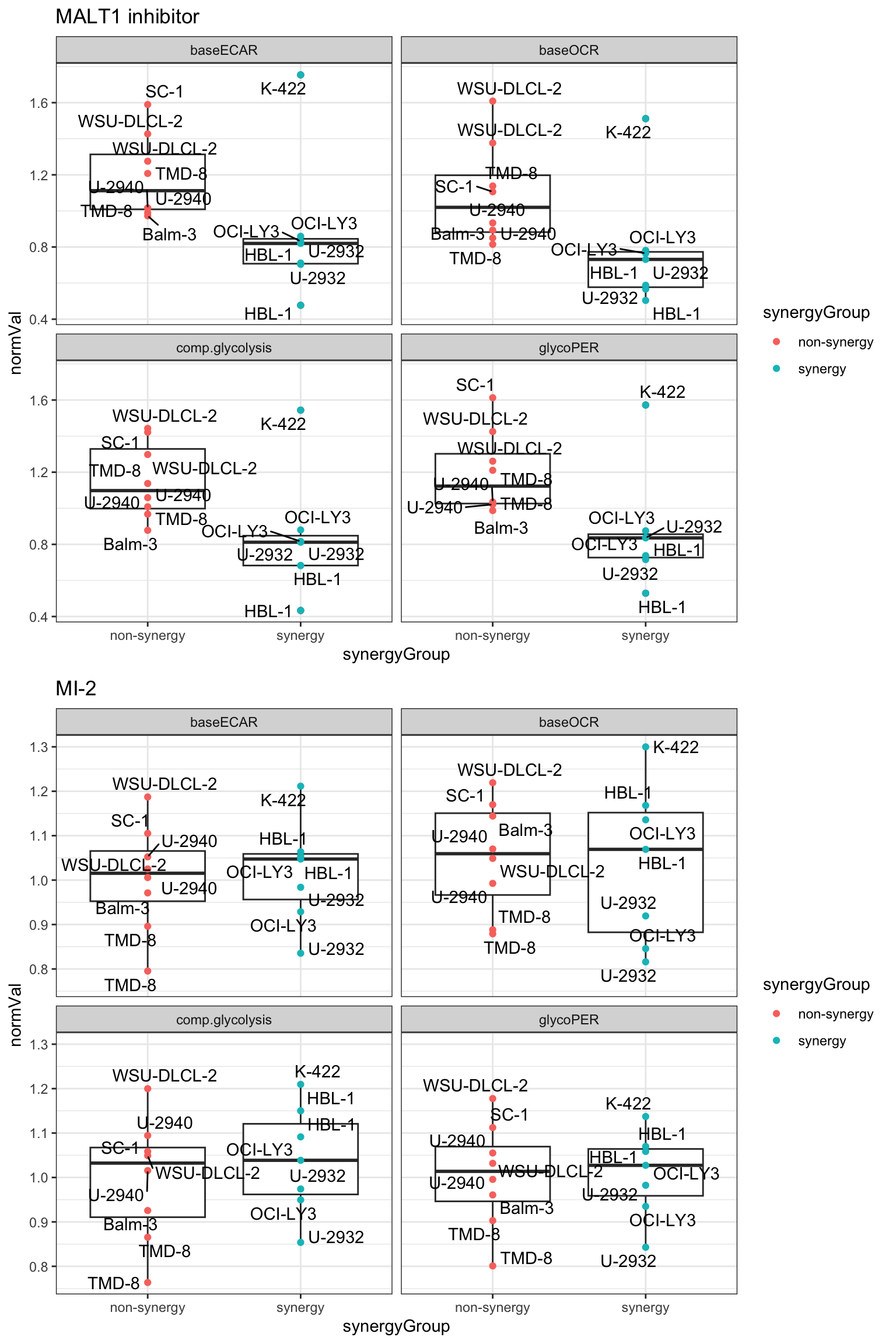 Looks like K-422 act as an outlier
T-test
testRes <- group_by(normTab, measure, Drug) %>% nest() %>%
  mutate(m = map(data, ~t.test(normVal ~ synergyGroup,.))) %>%
  mutate(res = map(m, broom::tidy)) %>%
  unnest(res) %>% select(measure, Drug, estimate, p.value) %>%
  arrange(p.value)
testRes
# A tibble: 8 × 4
# Groups: measure, Drug [8]
measure Drug estimate p.value
<chr> <chr> <dbl> <dbl>
1 glycoPER MALT1 inhibitor 0.326 0.0515
2 comp.glycolysis MALT1 inhibitor 0.316 0.0630
3 baseOCR MALT1 inhibitor 0.312 0.0796
4 baseECAR MALT1 inhibitor 0.307 0.110
5 comp.glycolysis MI-2 -0.0417 0.548
6 baseECAR MI-2 -0.0131 0.836
7 baseOCR MI-2 0.0152 0.856
8 glycoPER MI-2 -0.00295 0.959 No significant results
T-test (without K-422)
testRes <- filter(normTab, cellLine!="K-422") %>%
  group_by(measure, Drug) %>% nest() %>%
  mutate(m = map(data, ~t.test(normVal ~ synergyGroup,.))) %>%
  mutate(res = map(m, broom::tidy)) %>%
  unnest(res) %>% select(measure, Drug, estimate, p.value) %>%
  arrange(p.value)
testRes
# A tibble: 8 × 4
# Groups: measure, Drug [8]
measure Drug estimate p.value
<chr> <chr> <dbl> <dbl>
1 glycoPER MALT1 inhibitor 0.442 0.000665
2 baseECAR MALT1 inhibitor 0.453 0.000730
3 comp.glycolysis MALT1 inhibitor 0.434 0.000945
4 baseOCR MALT1 inhibitor 0.434 0.00281
5 baseOCR MI-2 0.0592 0.457
6 glycoPER MI-2 0.0186 0.739
7 baseECAR MI-2 0.0192 0.740
8 comp.glycolysis MI-2 -0.0131 0.845 Without K-422, Malt1 inhibitor has significant effect
sessionInfo()R version 4.2.0 (2022-04-22)
Platform: x86_64-apple-darwin17.0 (64-bit)
Running under: macOS Big Sur/Monterey 10.16
Matrix products: default
BLAS: /Library/Frameworks/R.framework/Versions/4.2/Resources/lib/libRblas.0.dylib
LAPACK: /Library/Frameworks/R.framework/Versions/4.2/Resources/lib/libRlapack.dylib
locale:
[1] en_US.UTF-8/en_US.UTF-8/en_US.UTF-8/C/en_US.UTF-8/en_US.UTF-8
attached base packages:
[1] stats graphics grDevices utils datasets methods base
other attached packages:
[1] gridExtra_2.3 forcats_0.5.1 stringr_1.4.1 dplyr_1.1.4.9000
[5] purrr_0.3.4 readr_2.1.2 tidyr_1.2.0 tibble_3.2.1
[9] ggplot2_3.4.1 tidyverse_1.3.2
loaded via a namespace (and not attached):
[1] readxl_1.4.0 backports_1.4.1
[3] fastmatch_1.1-3 drc_3.0-1
[5] jyluMisc_0.1.5 workflowr_1.7.0
[7] igraph_1.3.4 shinydashboard_0.7.2
[9] splines_4.2.0 BiocParallel_1.30.3
[11] GenomeInfoDb_1.32.2 TH.data_1.1-1
[13] digest_0.6.30 htmltools_0.5.4
[15] fansi_1.0.6 magrittr_2.0.3
[17] googlesheets4_1.0.0 cluster_2.1.3
[19] tzdb_0.3.0 limma_3.52.2
[21] modelr_0.1.8 matrixStats_0.62.0
[23] sandwich_3.0-2 piano_2.12.0
[25] colorspace_2.0-3 ggrepel_0.9.1
[27] rvest_1.0.2 haven_2.5.0
[29] xfun_0.31 crayon_1.5.2
[31] RCurl_1.98-1.7 jsonlite_1.8.3
[33] survival_3.4-0 zoo_1.8-10
[35] glue_1.7.0 survminer_0.4.9
[37] gtable_0.3.0 gargle_1.2.0
[39] zlibbioc_1.42.0 XVector_0.36.0
[41] DelayedArray_0.22.0 car_3.1-0
[43] BiocGenerics_0.42.0 abind_1.4-5
[45] scales_1.2.0 mvtnorm_1.1-3
[47] DBI_1.1.3 relations_0.6-12
[49] rstatix_0.7.0 Rcpp_1.0.9
[51] plotrix_3.8-2 xtable_1.8-4
[53] km.ci_0.5-6 stats4_4.2.0
[55] DT_0.23 htmlwidgets_1.5.4
[57] httr_1.4.3 fgsea_1.22.0
[59] gplots_3.1.3 ellipsis_0.3.2
[61] farver_2.1.1 pkgconfig_2.0.3
[63] sass_0.4.2 dbplyr_2.2.1
[65] utf8_1.2.4 labeling_0.4.2
[67] tidyselect_1.2.1 rlang_1.1.3
[69] later_1.3.0 munsell_0.5.0
[71] cellranger_1.1.0 tools_4.2.0
[73] visNetwork_2.1.0 cachem_1.0.6
[75] cli_3.6.2 generics_0.1.3
[77] broom_1.0.0 evaluate_0.15
[79] fastmap_1.1.0 yaml_2.3.5
[81] knitr_1.39 fs_1.5.2
[83] survMisc_0.5.6 caTools_1.18.2
[85] mime_0.12 slam_0.1-50
[87] xml2_1.3.3 compiler_4.2.0
[89] rstudioapi_0.13 beeswarm_0.4.0
[91] ggsignif_0.6.3 marray_1.74.0
[93] reprex_2.0.1 bslib_0.4.1
[95] stringi_1.7.8 highr_0.9
[97] lattice_0.20-45 Matrix_1.5-4
[99] KMsurv_0.1-5 shinyjs_2.1.0
[101] vctrs_0.6.5 pillar_1.9.0
[103] lifecycle_1.0.4 jquerylib_0.1.4
[105] data.table_1.14.8 cowplot_1.1.1
[107] bitops_1.0-7 httpuv_1.6.6
[109] GenomicRanges_1.48.0 R6_2.5.1
[111] promises_1.2.0.1 KernSmooth_2.23-20
[113] writexl_1.4.0 vipor_0.4.5
[115] IRanges_2.30.0 codetools_0.2-18
[117] MASS_7.3-58 gtools_3.9.3
[119] exactRankTests_0.8-35 assertthat_0.2.1
[121] SummarizedExperiment_1.26.1 rprojroot_2.0.3
[123] withr_3.0.0 multcomp_1.4-19
[125] S4Vectors_0.34.0 GenomeInfoDbData_1.2.8
[127] parallel_4.2.0 hms_1.1.1
[129] grid_4.2.0 rmarkdown_2.14
[131] MatrixGenerics_1.8.1 carData_3.0-5
[133] googledrive_2.0.0 git2r_0.30.1
[135] maxstat_0.7-25 ggpubr_0.4.0
[137] sets_1.0-21 Biobase_2.56.0
[139] shiny_1.7.4 lubridate_1.8.0
[141] ggbeeswarm_0.6.0