Pre-processing and quality control of the DLBCL combinatorial screen
Junyan Lu
2022-04-25
Last updated: 2022-12-19
Checks: 5 1
Knit directory: combiDLBCL/analysis/
This reproducible R Markdown analysis was created with workflowr (version 1.7.0). The Checks tab describes the reproducibility checks that were applied when the results were created. The Past versions tab lists the development history.
Great job! The global environment was empty. Objects defined in the global environment can affect the analysis in your R Markdown file in unknown ways. For reproduciblity it’s best to always run the code in an empty environment.
The command set.seed(20220425) was run prior to running
the code in the R Markdown file. Setting a seed ensures that any results
that rely on randomness, e.g. subsampling or permutations, are
reproducible.
Great job! Recording the operating system, R version, and package versions is critical for reproducibility.
Nice! There were no cached chunks for this analysis, so you can be confident that you successfully produced the results during this run.
Great job! Using relative paths to the files within your workflowr project makes it easier to run your code on other machines.
Tracking code development and connecting the code version to the
results is critical for reproducibility. To start using Git, open the
Terminal and type git init in your project directory.
This project is not being versioned with Git. To obtain the full
reproducibility benefits of using workflowr, please see
?wflow_start.
Load libraries and datasets
Quality Control
Basic screen information
How many combi drugs
unique(Combi.Screen$Drug_A) [1] "Lonidamin" "DMSO" "Teriflunomide"
[4] "NIKi" "Nutlin_3a" "Ciprofloxacin"
[7] "Venetoclax" "AZD3965" "Fluvastatin"
[10] "L_Methioninsulfoximin" "9_ING_41" "MK_2206"
[13] "OT_82" "DS18561882" "AZD7762"
[16] "Bafilomycin" "IACS_010759" "Ibrutinib"
[19] "SHIN1" "Dorsomorphin" "FCCP"
[22] "Everolimus" "Methotrexat" "CPI_613"
[25] "CK37" "Etoxomir" "V_9302"
[28] "OTX015" "CB_839" "BAY_876"
[31] "C75" What are the anchor drugs
unique(Combi.Screen$Drug_B)[1] "CHOP" "DMSO" "NIK_SIM1" "B022" "CHP_Pola"
[6] "CHP" "Polatuzumab"Plot plate layout
screenData <- Combi.Screen %>%
    mutate(type = case_when(
        Drug_A == "DMSO" & Drug_B == "DMSO" ~ "DMSO",
        Drug_A == "DMSO" & Drug_B != "DMSO" ~ "base_only",
        Drug_A != "DMSO" & (Drug_B == "DMSO" | Drug_B.Conc ==0) ~ "drug_only",
        TRUE ~ "combine"
    )) %>% mutate(plateID = paste0(Name, "_", Plate)) %>%
    mutate(ifEdge = Row %in% c("A","B","O","P") | Column.x %in% c("01","02","23","24"))
The two most outside layer is defined as edges.
Does every plate have the same layout?
plateIden <- group_by(screenData, plateID, Well) %>%
    summarise(ifSame = length(unique(Drug_A))==1 &
                  length(unique(Drug_B))==1)
`summarise()` has grouped output by 'plateID'. You can override using the
`.groups` argument.all(plateIden$ifSame)[1] TRUEYes.
Plot drug type layout
plateLayout <- distinct(screenData, Row, Column.x, Drug_A, Drug_B, Plate, type)

ggplot(plateLayout, aes(x=Column.x, y=Row, fill = type)) +
    geom_tile() +
    theme_classic() +
    facet_wrap(~Plate, ncol = 1)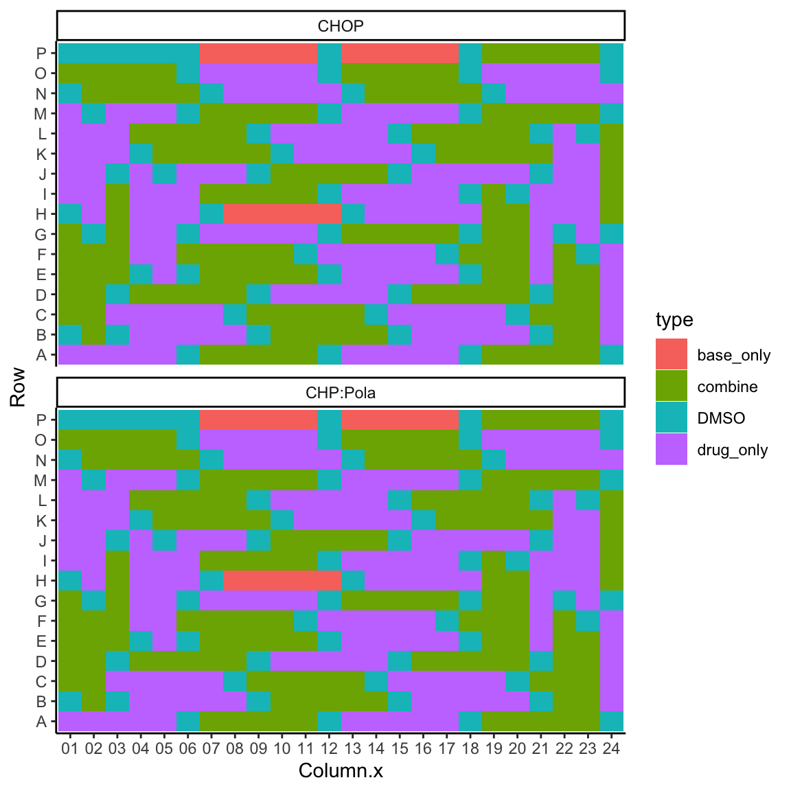
Plot Base drug layout
ggplot(plateLayout, aes(x=Column.x, y=Row, fill = Drug_B)) +
    geom_tile() +
    theme_classic() +
    facet_wrap(~Plate, ncol = 1)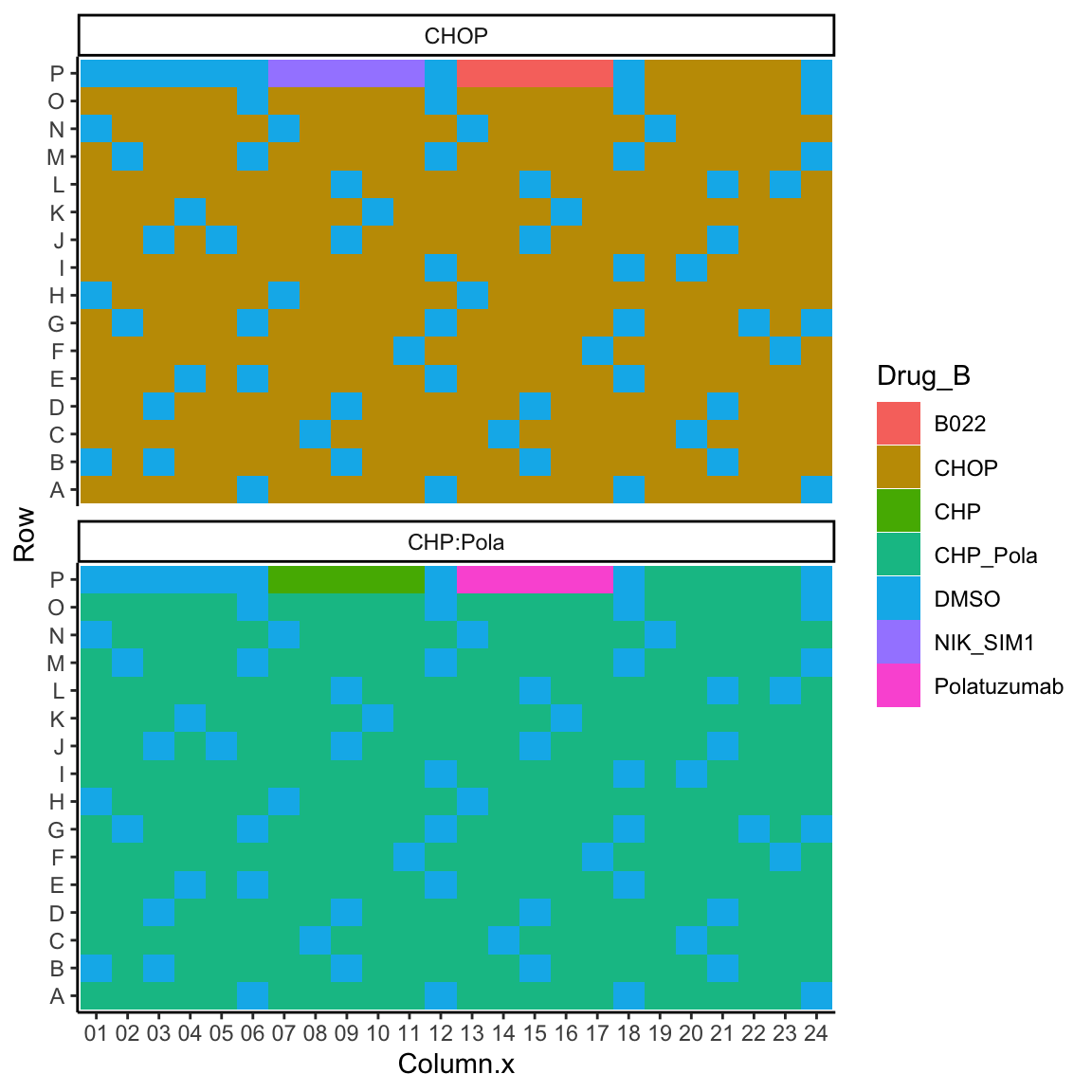
Plot combi drug layout
ggplot(plateLayout, aes(x=Column.x, y=Row, fill = Drug_A)) +
    geom_tile() +
    theme_classic() +
    facet_wrap(~Plate, ncol = 1)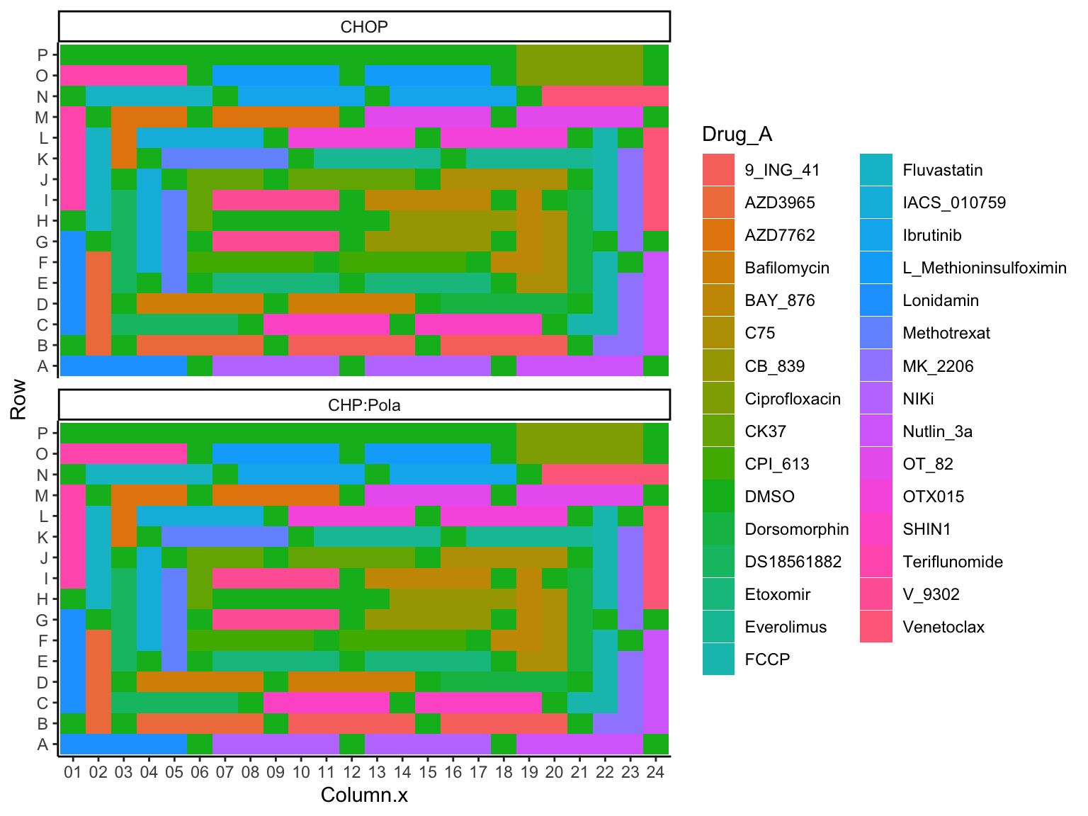
Viability plate plot
Normalize plate by internal DMSO wells
dmsoVal <- filter(screenData, type == "DMSO", !ifEdge) %>%
    group_by(plateID) %>%
    summarise(medDMSO = median(Count))
screenData <- left_join(screenData, dmsoVal, by ="plateID") %>%
    mutate(normVal = Count/medDMSO)
pList <- lapply(unique(screenData$plateID), function(id){
plotTab <- filter(screenData, plateID == id)
ggplot(plotTab, aes(x=Column.x, y=Row, fill = normVal)) +
geom_tile() +
scale_fill_gradient2(low = "blue", high = "red", mid = "white", midpoint = 1,limits=c(0,2)) +
theme_classic() +
ggtitle(id)
})
jyluMisc::makepdf(pList, "../docs/plate_plot.pdf",ncol = 2, nrow = 3, width = 12, height = 12)Loading required package: gridExtra
Attaching package: 'gridExtra'The following object is masked from 'package:dplyr':
combineCheck DMSO controls
Mean and Variance of internal controls
plotTab <- filter(screenData, !ifEdge, type == "DMSO")
ggplot(plotTab, aes(x=Name, y=Count, col = Plate)) +
    ggbeeswarm::geom_quasirandom() +
    theme(axis.text.x = element_text(angle = 90, vjust=0.5, hjust = 1))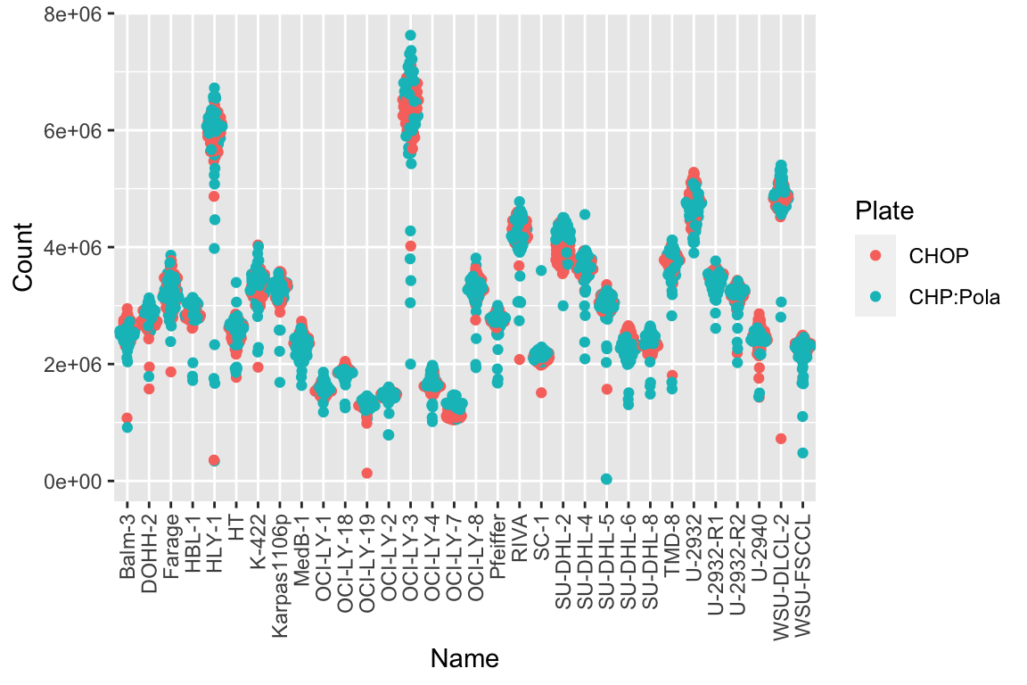
Visualize edge effect
plotTab <- screenData %>% filter(type == "DMSO")
ggplot(plotTab, aes(x=Name, y=normVal, col = ifEdge)) +
geom_boxplot() +
theme(axis.text.x = element_text(angle = 90, vjust=0.5, hjust = 1))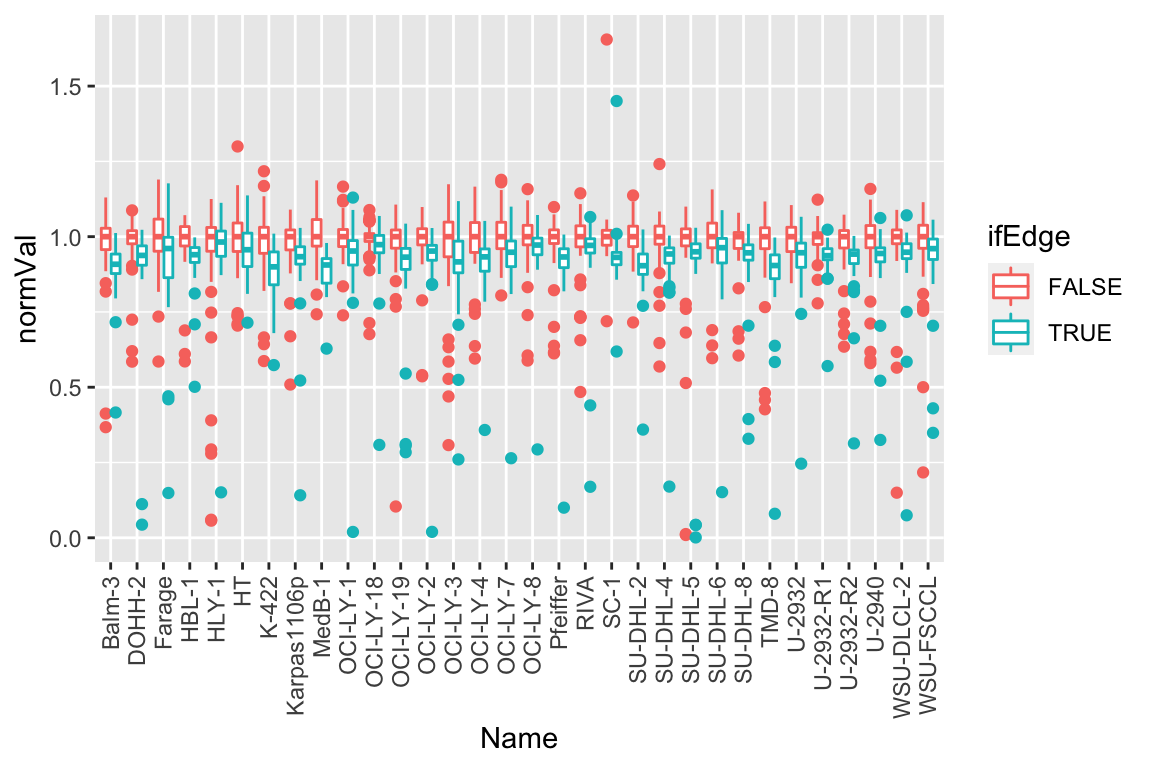 Some degree of edge effect can be observed
Edge effect
plotTab <- screenData %>% filter(type == "DMSO")
ggplot(plotTab, aes(x=Row, y=normVal)) +
    geom_boxplot() +
    theme(axis.text.x = element_text(angle = 90, vjust=0.5, hjust = 1))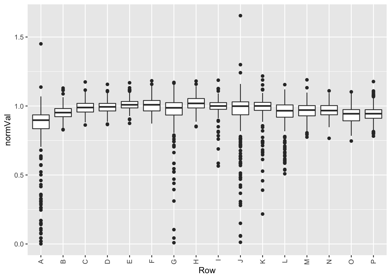
plotTab <- screenData %>% filter(type == "DMSO")
ggplot(plotTab, aes(x=Column.x, y=normVal)) +
    geom_boxplot() +
    theme(axis.text.x = element_text(angle = 90, vjust=0.5, hjust = 1))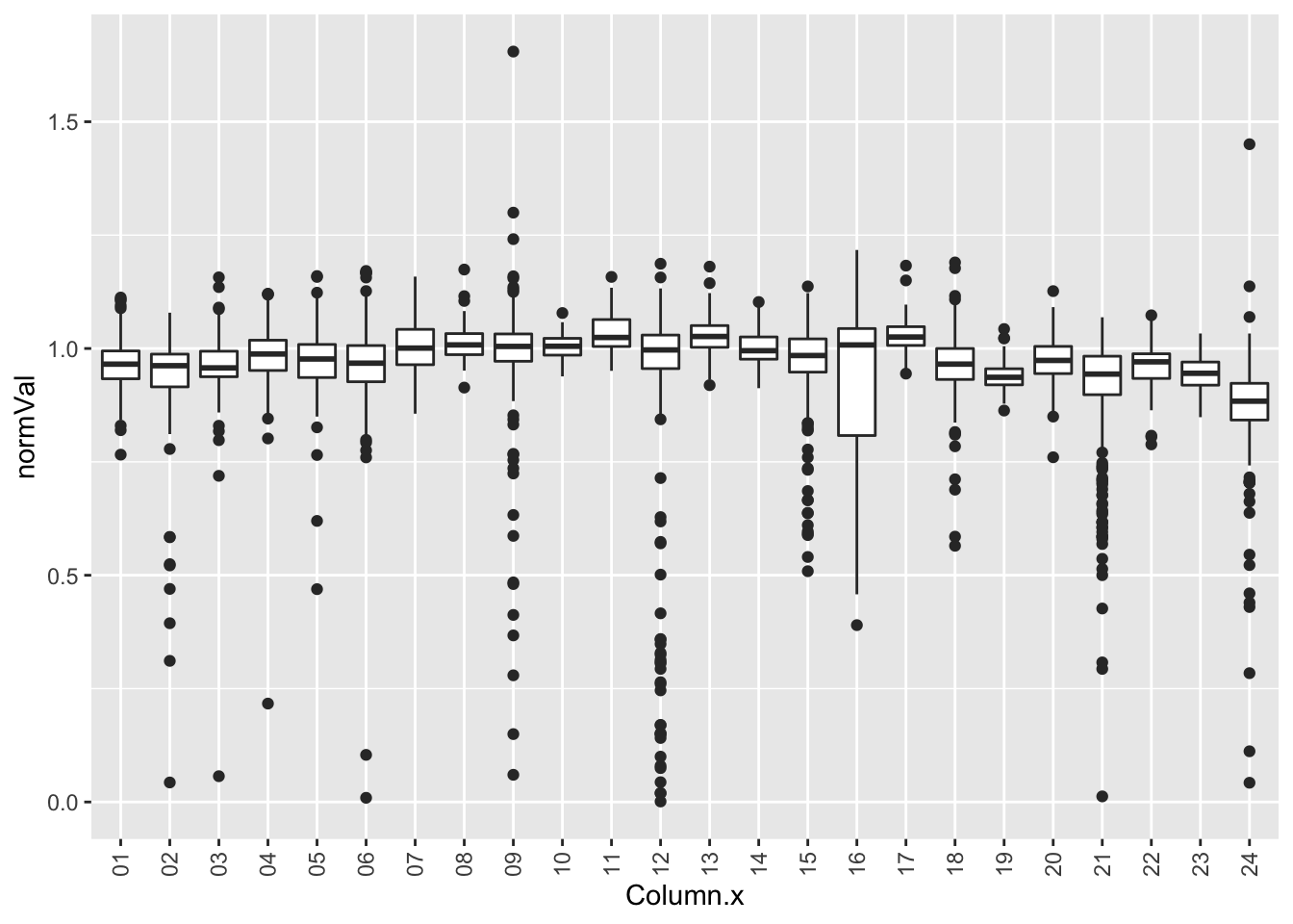
Why some DMSO wells have very low viability
problemPlates <- filter(screenData, type == "DMSO", normVal < 0.5)
problemPlates %>% mutate_if(is.numeric, formatC, digits=0) %>% DT::datatable()
Any patterns?
table(problemPlates$Well, problemPlates$Plate)
      CHOP CHP:Pola
  A12    0       26
  A24    0        5
  G02    1        3
  G06    1        1
  G24    1        0
  J03    0        1
  J05    0        1
  J09    5        2
  J21    0        4
  K04    0        1
  K16    0        2
a12Well <- filter(screenData, Well == "A12")
ggplot(a12Well, aes(x=Plate, y=normVal)) +
geom_boxplot() + geom_point()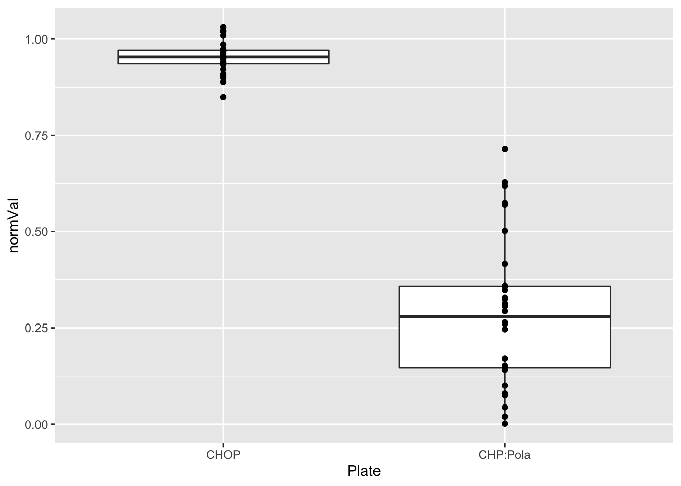
Visualize Combination design
drugTab <- distinct(screenData, Drug_A, Drug_B, Drug_A.Conc, Drug_B.Conc) %>%
  mutate(present = 1) %>%
  mutate(drugConcA = paste0(Drug_A,"_",Drug_A.Conc),
         drugConcB = paste0(Drug_B, "_", Drug_B.Conc))


countTab <- group_by(screenData, Drug_A, Drug_B, Drug_A.Conc, Drug_B.Conc, Name) %>%
  summarise(n=length(Drug_A)) %>%
  filter(! (Drug_B=="DMSO" & Drug_A == "DMSO"), n>1)
`summarise()` has grouped output by 'Drug_A', 'Drug_B', 'Drug_A.Conc',
'Drug_B.Conc'. You can override using the `.groups` argument.orderA <- arrange(drugTab, Drug_A, Drug_A.Conc)
orderB <- arrange(drugTab, Drug_B, Drug_B.Conc)
designMat <- drugTab %>%
select(drugConcA, drugConcB, present) %>%
pivot_wider(names_from = drugConcB, values_from = present) %>%
pivot_longer(-drugConcA) %>%
mutate(name = factor(name, levels = unique(orderB$drugConcB)),
drugConcA = factor(drugConcA, levels = unique(orderA$drugConcA)))
ggplot(designMat, aes(x=name, y=drugConcA, fill = value)) +
geom_tile() +
theme_minimal() +
theme(axis.text.x = element_text(angle = 90, hjust = 1, vjust=0.5))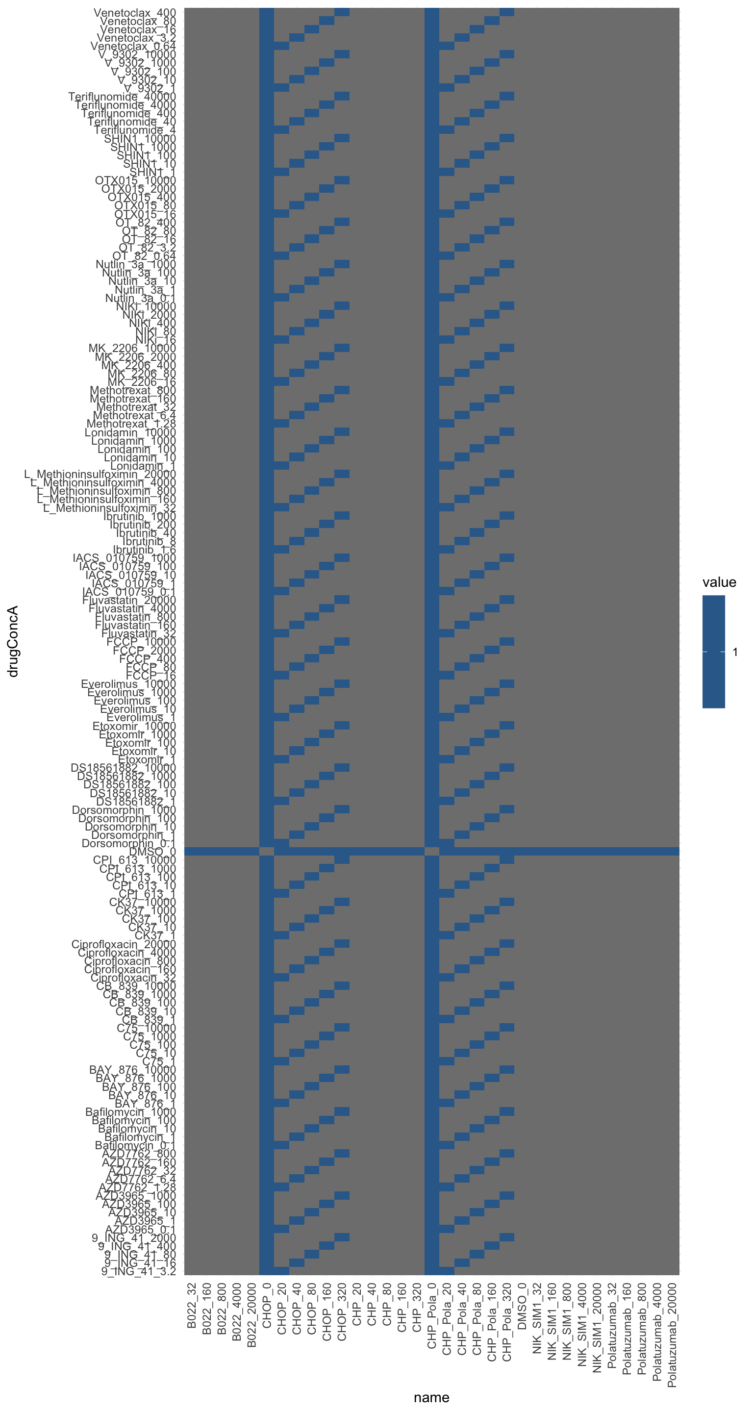 It follows diagonal design.
Visualize single drug effect
Dose response curves of single agent drugs
drugTab <- distinct(screenData, Drug_A, Drug_B, Drug_B.Conc) %>%
  filter(Drug_A != "DMSO", Drug_B.Conc==0) %>%
  mutate(id = paste0(Drug_A,"_",Drug_B,"_",Drug_B.Conc))

pList.single <- lapply(seq(nrow(drugTab)), function(i) {
  rec <- drugTab[i,]
  plotTab <- filter(screenData,
                    Drug_A == rec$Drug_A,
                    Drug_B == rec$Drug_B,
                    Drug_B.Conc == rec$Drug_B.Conc)

  ggplot(plotTab, aes(x=Drug_A.Conc, y=normVal, group = Name, col = Name)) +
    geom_line() + geom_point() +
    scale_x_log10() + theme_bw() +
    coord_cartesian(ylim = c(0,1.5)) +
    ggtitle(rec$id) +
    theme(legend.position = "none")
})
names(pList.single) <- drugTab$id

jyluMisc::makepdf(pList.single, "../docs/DoseResponse_single.pdf",2,3,width = 8, height = 8)Dose response curves of base drugs
drugTab <- distinct(screenData, Drug_A, Drug_B) %>%
  filter(Drug_A == "DMSO", Drug_B!= "DMSO")

pList.base <- lapply(seq(nrow(drugTab)), function(i) {
  rec <- drugTab[i,]
  plotTab <- filter(screenData,
                    Drug_A == rec$Drug_A,
                    Drug_B == rec$Drug_B)

  ggplot(plotTab, aes(x=Drug_B.Conc, y=normVal, group = Name, col = Name)) +
    geom_line() + geom_point() +
    scale_x_log10() + theme_bw() +
    coord_cartesian(ylim = c(0,1.5)) +
    ggtitle(paste0(rec$Drug_B)) +
    theme(legend.position = "none")
})
names(pList.base) <- drugTab$Drug_B

jyluMisc::makepdf(pList.base, "../docs/DoseResponse_base.pdf",2,3,width = 8, height = 8)Some drugs show strange dose-response curves
MK-2206
cowplot::plot_grid(pList.single$MK_2206_CHOP_0, pList.single$MK_2206_CHP_Pola_0)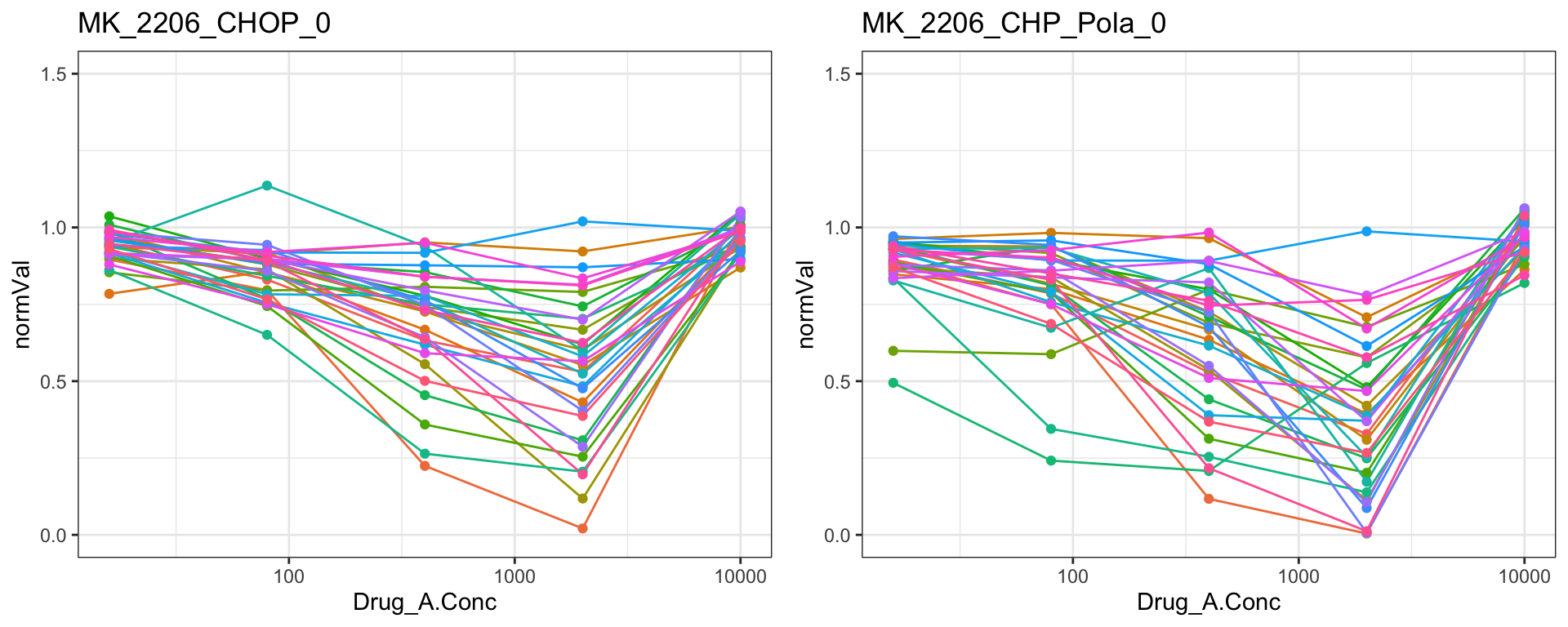
Methotrexat
cowplot::plot_grid(pList.single$Methotrexat_CHOP_0, pList.single$Methotrexat_CHP_Pola_0)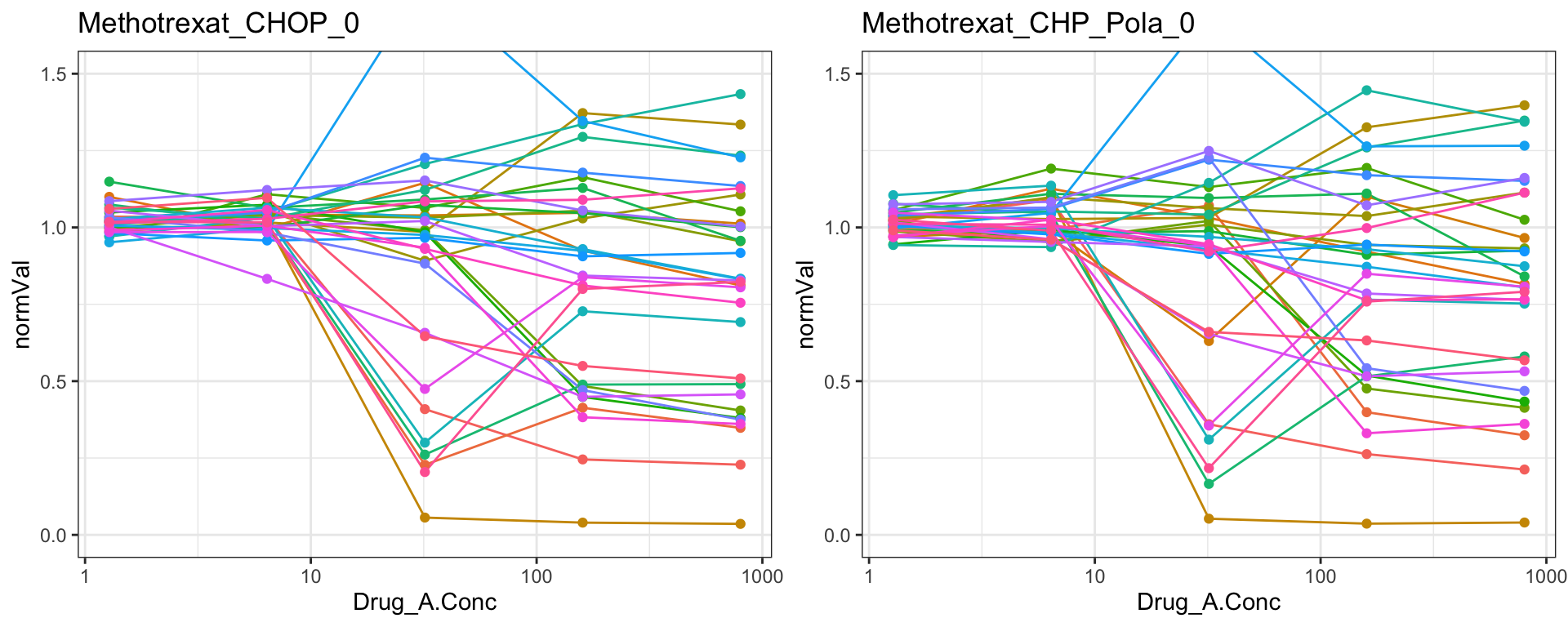
C75
cowplot::plot_grid(pList.single$C75_CHOP_0, pList.single$C75_CHP_Pola_0)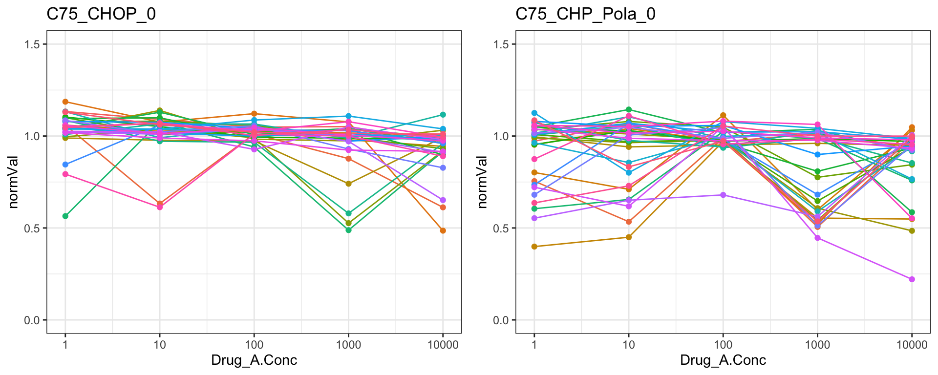
FCCP
cowplot::plot_grid(pList.single$FCCP_CHOP_0, pList.single$FCCP_CHP_Pola_0)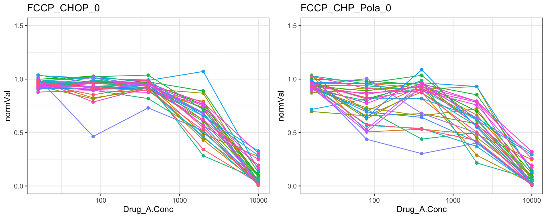
Remove those four drugs from the dataset
problemDrugs <- c("MK_2206","Methotrexat","C75","FCCP")
screenData <- filter(screenData, ! Drug_A %in% problemDrugs)
Save the data object for downstream analyses
save(screenData, file = "../output/screenData.RData")Analysis of CHOP screen from previous results
The CHOP single agent screen may have not worked in this combinatorial screen. Compare the current screen with previous screen to see if it’s possible to use the data from previous screen
load("../data/CHOP_screen_all_data.RData")

CHOP_Screen_data <- CHOP_Screen_data %>%
  mutate(Drug_Conc = as.numeric(Drug_Conc),
         Name = str_replace_all(Name, "_", "-"))
Dose response of CHOP
plotTab <- CHOP_Screen_data
p <- ggplot(plotTab, aes(x=Drug_Conc, y=Normalized_values, group = Name, col = Name)) +
geom_line() + geom_point() +
scale_x_log10() + theme_bw() +
coord_cartesian(ylim = c(0,1.5)) +
#ggtitle(paste0(rec$Drug_B)) +
theme(legend.position = "right") +
facet_wrap(~drug, scales = "free_x")
p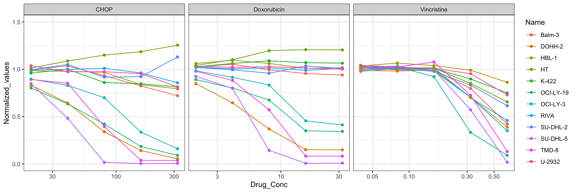 The CHOP data here looks fine.
Compare the CHOP data from the old screen to the CHP-Pola data from the new screen.
Get CHP-Pola single agent
screenCHP <- filter(screenData, Drug_B == "CHP_Pola", Drug_A == "DMSO") %>%
  select(Name, normVal, Drug_B.Conc) %>%
  dplyr::rename(viabCHP = normVal)

screenCombine <- CHOP_Screen_data %>%
  filter(drug == "CHOP") %>%
  select(Name, Drug_Conc, Normalized_values) %>%
  dplyr::rename(viabCHOP = Normalized_values) %>%
  full_join(screenCHP, by =c(Name = "Name",Drug_Conc = "Drug_B.Conc"))
Visualize data completeness
comTab <- screenCombine %>%
  mutate(status = case_when(
    !is.na(viabCHOP) & !is.na(viabCHP) ~ "both",
    !is.na(viabCHOP) & is.na(viabCHP) ~ "CHOP only",
    is.na(viabCHOP) & !is.na(viabCHP) ~ "CHP:Pola only",
  ))

ggplot(comTab, aes(x=factor(Drug_Conc), y = Name, fill = status)) +
  geom_tile(col = "grey")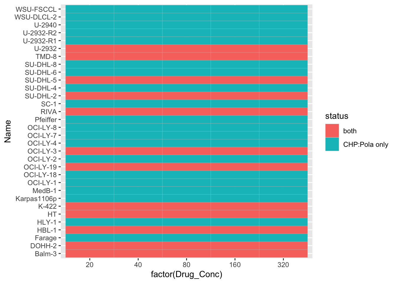
Compare reproducibility per concentration
ggplot(screenCombine, aes(x=viabCHOP, y = viabCHP)) +
  geom_point(aes(col = Name)) + facet_wrap(~Drug_Conc) + scale_x_log10() +
  xlim(0,1.5) + ylim(0,1.5) +
  geom_smooth(method = "lm")
Scale for 'x' is already present. Adding another scale for 'x', which will
replace the existing scale.`geom_smooth()` using formula 'y ~ x'Warning: Removed 100 rows containing non-finite values (stat_smooth).Warning: Removed 100 rows containing missing values (geom_point).Warning: Removed 22 rows containing missing values (geom_smooth).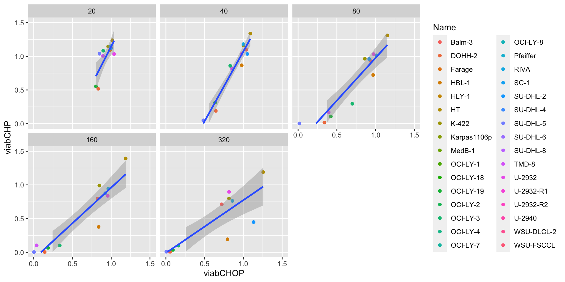
Similarity of dose response sample
plotTab <- screenCombine %>%
  pivot_longer(-c("Name","Drug_Conc"),names_to = "drug", values_to = "viab")
ggplot(plotTab, aes(x=Drug_Conc, y=viab, col = drug, group = drug)) +
  geom_line() + geom_point() +
  facet_wrap(~Name, ncol=3) +
  scale_x_log10()
Warning: Removed 25 row(s) containing missing values (geom_path).Warning: Removed 100 rows containing missing values (geom_point).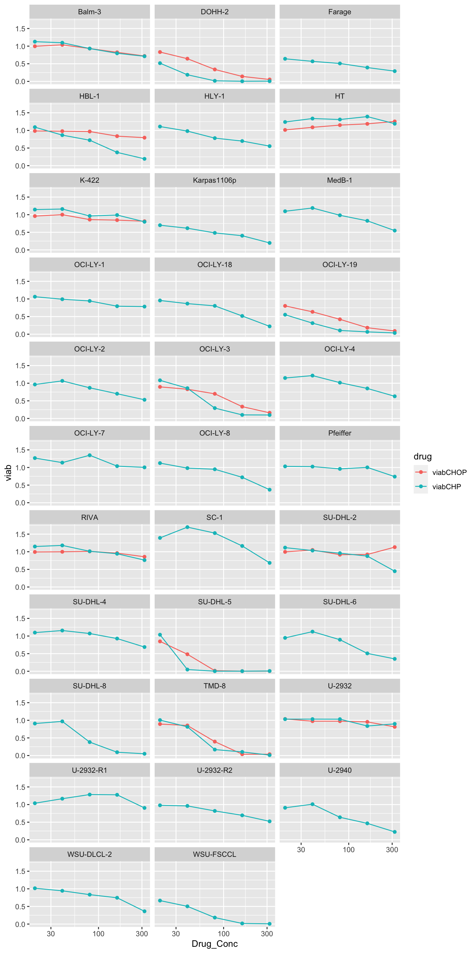
Does-response of overlapped cell lines
overCell <- unique(filter(comTab, status == "both")$Name)
plotCom <- filter(plotTab, Name %in% overCell)
ggplot(plotCom, aes(x=Drug_Conc, y=viab, col = Name)) +
geom_point() +
geom_line() +
facet_wrap(~drug) +
scale_x_log10()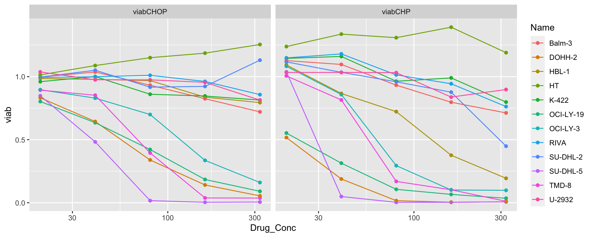 Two cell lines: Two cell lines, SU-DHL-2 and HBL-1, may be classified as
CHP resistant in the old screen data but CHP sensitive in the new screen
data.
Two cell lines: Two cell lines, SU-DHL-2 and HBL-1, may be classified as
CHP resistant in the old screen data but CHP sensitive in the new screen
data.
Does-response of cell lines in new screen only
overCell <- unique(filter(comTab, status == "CHP:Pola only")$Name)
plotCom <- filter(plotTab, Name %in% overCell) %>%
filter(drug == "viabCHP")
ggplot(plotCom, aes(x=Drug_Conc, y=viab, col = Name, group = Name)) +
geom_point() +
geom_line() +
scale_x_log10()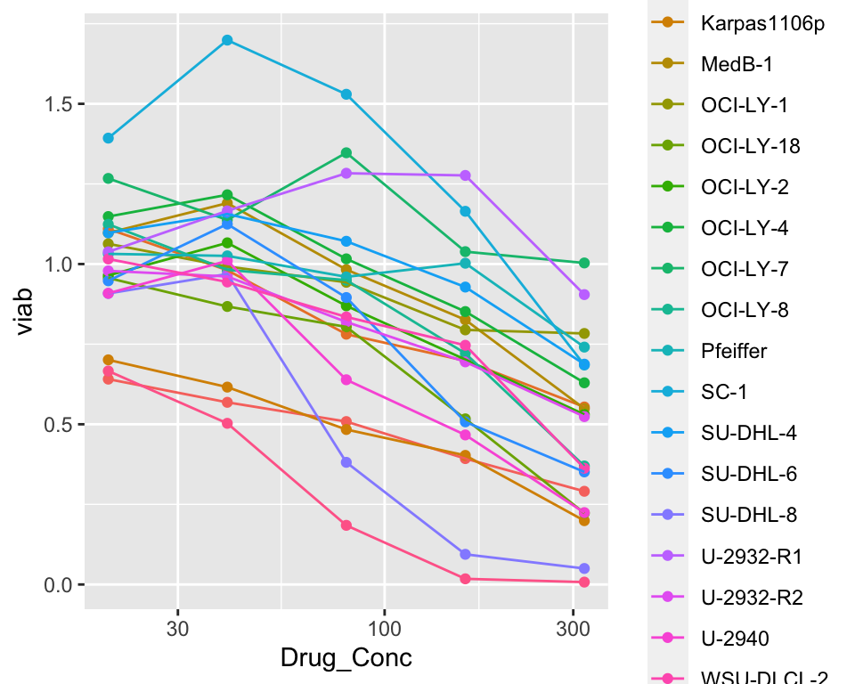 No clear separation.
Does-response of cell lines in new screen only (colored by TP53 mutational status)
load("../data/SVs_filtered.RData")
mutCell <- filter(svTab, Gene == "TP53")$Name
allCell <- unique(svTab$Name)
tp53Tab <- tibble(Name = allCell) %>%
  mutate(TP53 = ifelse(Name %in% mutCell, "Mut","WT"))

overCell <- unique(filter(comTab, status == "CHP:Pola only")$Name)

plotCom <- filter(plotTab, Name %in% overCell) %>%
  filter(drug == "viabCHP") %>%
  left_join(tp53Tab)
Joining, by = "Name"ggplot(plotCom, aes(x=Drug_Conc, y=viab, col = TP53, group = Name)) +
geom_point() +
geom_line() +
ggrepel::geom_text_repel(data = filter(plotCom, Drug_Conc == 320), aes(label = Name)) +
scale_x_log10() +
theme_bw()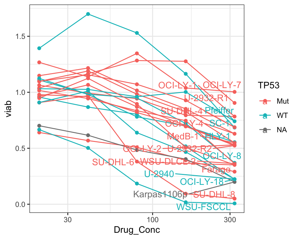
Check if drug combination effect are comparable between CHOP and CHP:Pola?
screenSub.com <- filter(screenData, Drug_B %in% c("CHP_Pola","CHOP")) %>%
  group_by(Name, Drug_A, Drug_B, Drug_A.Conc, Drug_B.Conc, Drug_A.ConcStep) %>%
  summarise(viab = normVal) %>% ungroup()
`summarise()` has grouped output by 'Name', 'Drug_A', 'Drug_B', 'Drug_A.Conc',
'Drug_B.Conc'. You can override using the `.groups` argument.pList <- lapply(sort(unique(screenSub.com$Drug_B.Conc)), function(conc) {
plotTab <- filter(screenSub.com, Drug_B.Conc == conc) %>%
select(-Drug_B.Conc) %>%
pivot_wider(names_from = Drug_B, values_from = viab) %>%
mutate(n1=length(CHOP), n2 = length(CHP_Pola))
ggplot(plotTab, aes(x=CHOP, y=CHP_Pola)) +
geom_point(aes(col = Drug_A.ConcStep)) + facet_wrap(~Drug_A) +
ggtitle(sprintf("Drug_B.Conc = %s",conc))
})
jyluMisc::makepdf(pList, "../docs/compare_CHOP_CHP.pdf", height = 10, width = 10, nrow = 1, ncol = 1)AUC reproducibility of single agent
aucTab <- filter(screenData, Drug_B.Conc == 0, Drug_B != "DMSO") %>%
  group_by(Name, Drug_A, Drug_B) %>%
  summarise(auc = calcAUC(normVal, Drug_A.Conc)) %>%
  pivot_wider(names_from = Drug_B, values_from = auc)
`summarise()` has grouped output by 'Name', 'Drug_A'. You can override using
the `.groups` argument.For each drug
ggplot(aucTab, aes(x=CHOP, y= CHP_Pola)) +
  geom_point() +
  facet_wrap(~Drug_A)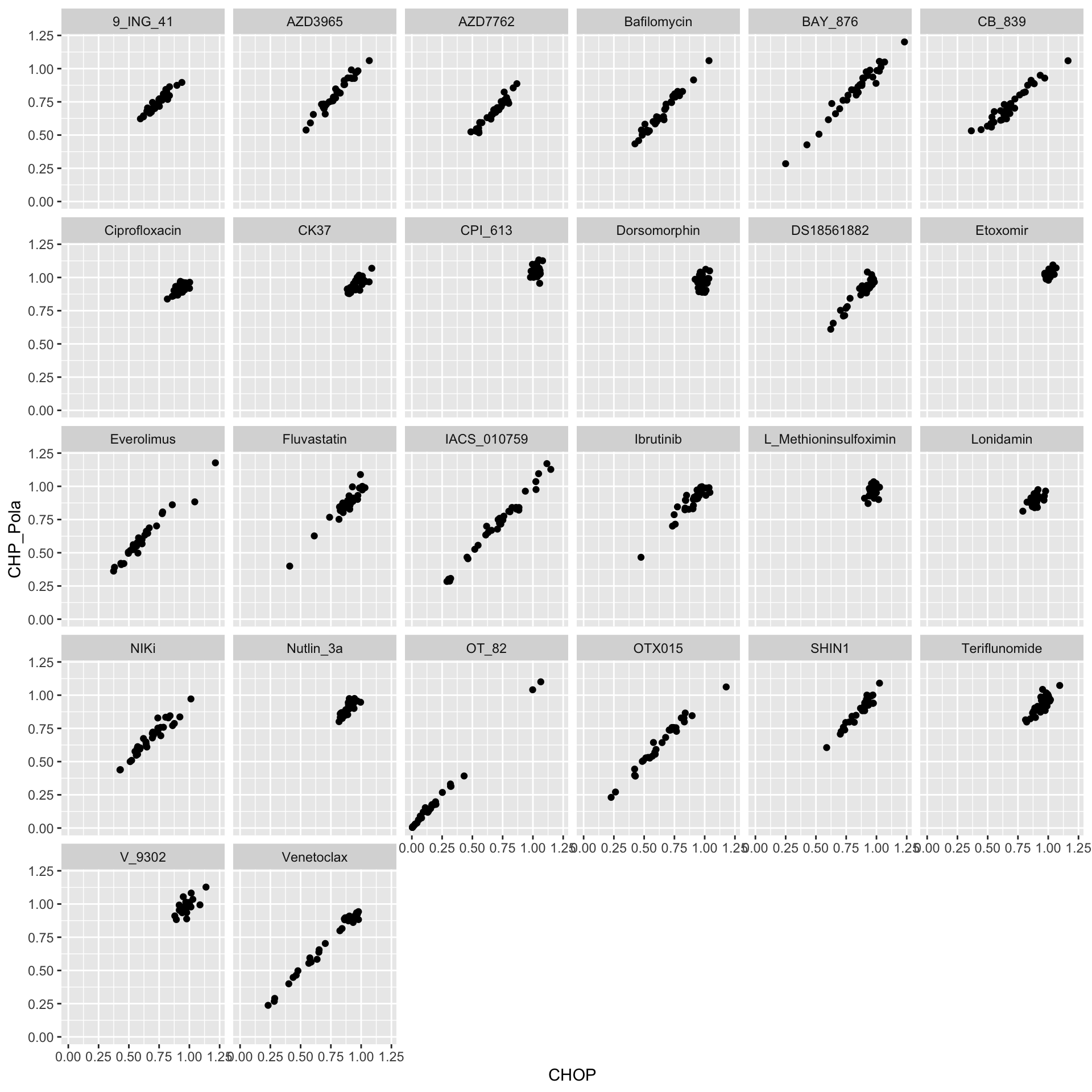
For each cell line
ggplot(aucTab, aes(x=CHOP, y= CHP_Pola)) +
  geom_point() +
  facet_wrap(~Name)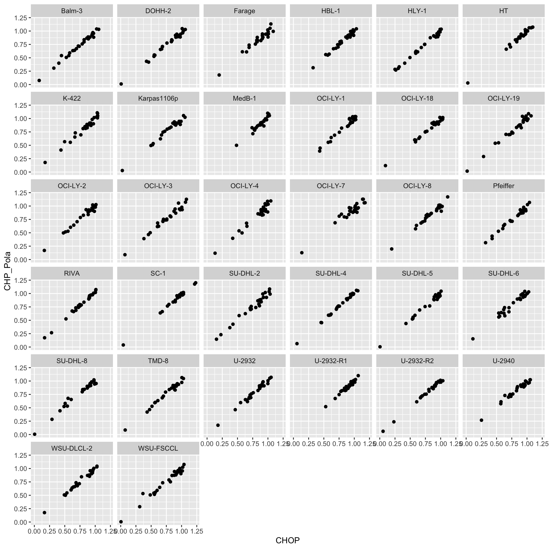
Compare with previous screen from Tobias
Load data
load("../data/Screen.CL19.RData")Subset for cell lines present in current screen
overCell <- intersect(Screen.CL19$Name, screenData$Name)
overCell
[1] "Farage" "OCI-LY-7" "HLY-1" "K-422" "OCI-LY-1"
[6] "WSU-DLCL-2" "RIVA" "U-2940" "SU-DHL-5" "OCI-LY-3"
[11] "SU-DHL-4" "Pfeiffer" "MedB-1" "SU-DHL-2" "WSU-FSCCL"
[16] "OCI-LY-4" "SU-DHL-8" "DOHH-2" "OCI-LY-18" "SC-1"
[21] "HBL-1" "OCI-LY-2" "U-2932-R2" "OCI-LY-19" "HT"
[26] "U-2932-R1" "SU-DHL-6" "OCI-LY-8" "Balm-3" "TMD-8"
[31] "U-2932" 31 cell lines can be found
Overlapped drugs
overDrug <- intersect(Screen.CL19$Drug, c(screenData$Drug_A, screenData$Drug_B))
overDrug
[1] "DMSO" "OTX015" "NIKi" "Venetoclax" "Ibrutinib"
[6] "Everolimus"overDrug <- overDrug[overDrug!="DMSO"]Reproducibility of common drugs and cell lines
Process the new screen data by Lea
newScreen <- filter(screenData, Drug_A %in% overDrug, Name %in% overCell, Drug_B.Conc ==0, Plate == "CHP:Pola") %>%
  group_by(Name, Drug_A, Drug_A.Conc) %>%
  summarise(normVal = mean(normVal, na.rm=TRUE)) %>%
  rename(Drug = Drug_A, conc = Drug_A.Conc)
`summarise()` has grouped output by 'Name', 'Drug_A'. You can override using
the `.groups` argument.aucTab <- newScreen %>% group_by(Name, Drug) %>%
summarise(auc = calcAUC(normVal, conc))`summarise()` has grouped output by 'Name'. You can override using the
`.groups` argument.newScreen <- newScreen %>% left_join(aucTab) %>%
mutate(screen = "LeaScreen")Joining, by = c("Name", "Drug")Process the old screen data by Tobias
oldScreen <- filter(Screen.CL19, Drug %in% overDrug, Name %in% overCell, TimePoint == "48 h") %>%
  dplyr::rename(normVal = Normalized, conc = Drug.Conc) %>%
  group_by(Name, Drug, conc) %>%
  summarise(normVal = mean(normVal, na.rm=TRUE))
`summarise()` has grouped output by 'Name', 'Drug'. You can override using the
`.groups` argument.aucTab <- oldScreen %>% group_by(Name, Drug) %>%
summarise(auc = calcAUC(normVal, conc))`summarise()` has grouped output by 'Name'. You can override using the
`.groups` argument.oldScreen <- oldScreen %>% left_join(aucTab) %>%
mutate(screen = "TobiasScreen")Joining, by = c("Name", "Drug")Plot dose response
screenTab.com <- bind_rows(newScreen, oldScreen) %>%
  filter(Drug %in% overDrug)

pList <- lapply(unique(screenTab.com$Name), function(cellLine) {
  plotTab <- filter(screenTab.com, Name == cellLine)
  ggplot(plotTab, aes(x=conc, y=normVal, col = Drug, linetype = screen)) +
    geom_point() + geom_line() +
    scale_x_log10() +
    ggtitle(cellLine) +
    theme_bw()
})
jyluMisc::makepdf(pList, "./compare_TobiaScreen_LeaScreen_doseResponse.pdf",
                  ncol=2, nrow =3, width = 10, height = 10)
Reproducibility of AUC per cell line
plotTab <- distinct(screenTab.com, Name, Drug, auc, screen) %>%
  pivot_wider(names_from = screen, values_from = auc)
ggplot(plotTab, aes(x=LeaScreen, y=TobiasScreen, label = Drug)) +
  geom_point(aes(col=Drug)) +
  ggrepel::geom_text_repel() +
  geom_smooth(method = "lm") +
  facet_wrap(~Name, ncol=3) +
  xlim(0,1.2) + ylim(0,1.2)
`geom_smooth()` using formula 'y ~ x'Warning: Removed 2 rows containing missing values (geom_smooth).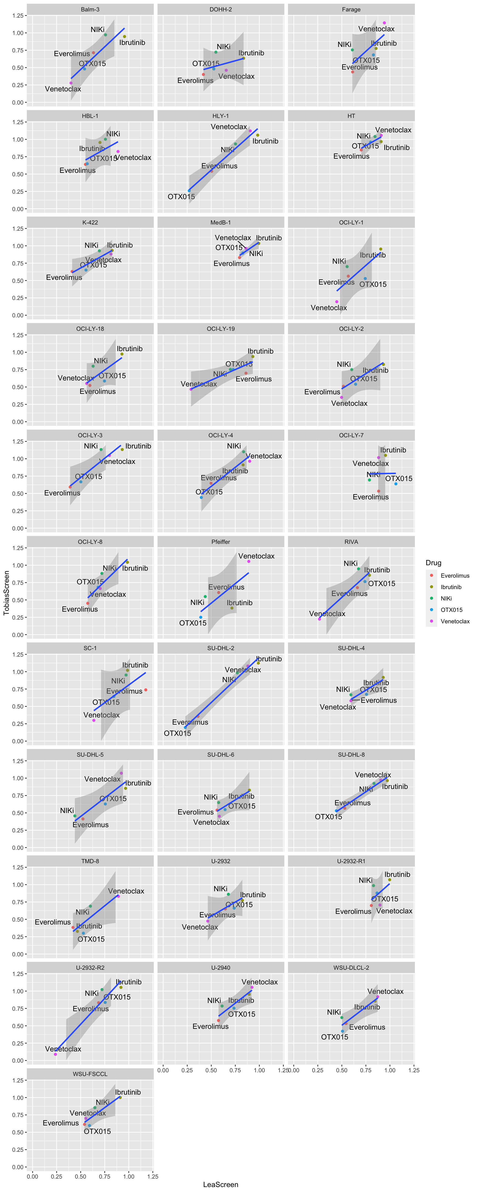
Reproducibility of AUC per drug
ggplot(plotTab, aes(x=LeaScreen, y=TobiasScreen,label = Name)) +
  geom_point(aes( col=Name)) +
  ggrepel::geom_text_repel() +
  geom_smooth(method = "lm") +
  facet_wrap(~Drug, ncol=2) +
    xlim(0,1.2) + ylim(0,1.2)
`geom_smooth()` using formula 'y ~ x'Warning: ggrepel: 14 unlabeled data points (too many overlaps). Consider
increasing max.overlapsWarning: ggrepel: 12 unlabeled data points (too many overlaps). Consider
increasing max.overlapsWarning: ggrepel: 6 unlabeled data points (too many overlaps). Consider
increasing max.overlapsWarning: ggrepel: 20 unlabeled data points (too many overlaps). Consider
increasing max.overlapsWarning: ggrepel: 4 unlabeled data points (too many overlaps). Consider
increasing max.overlaps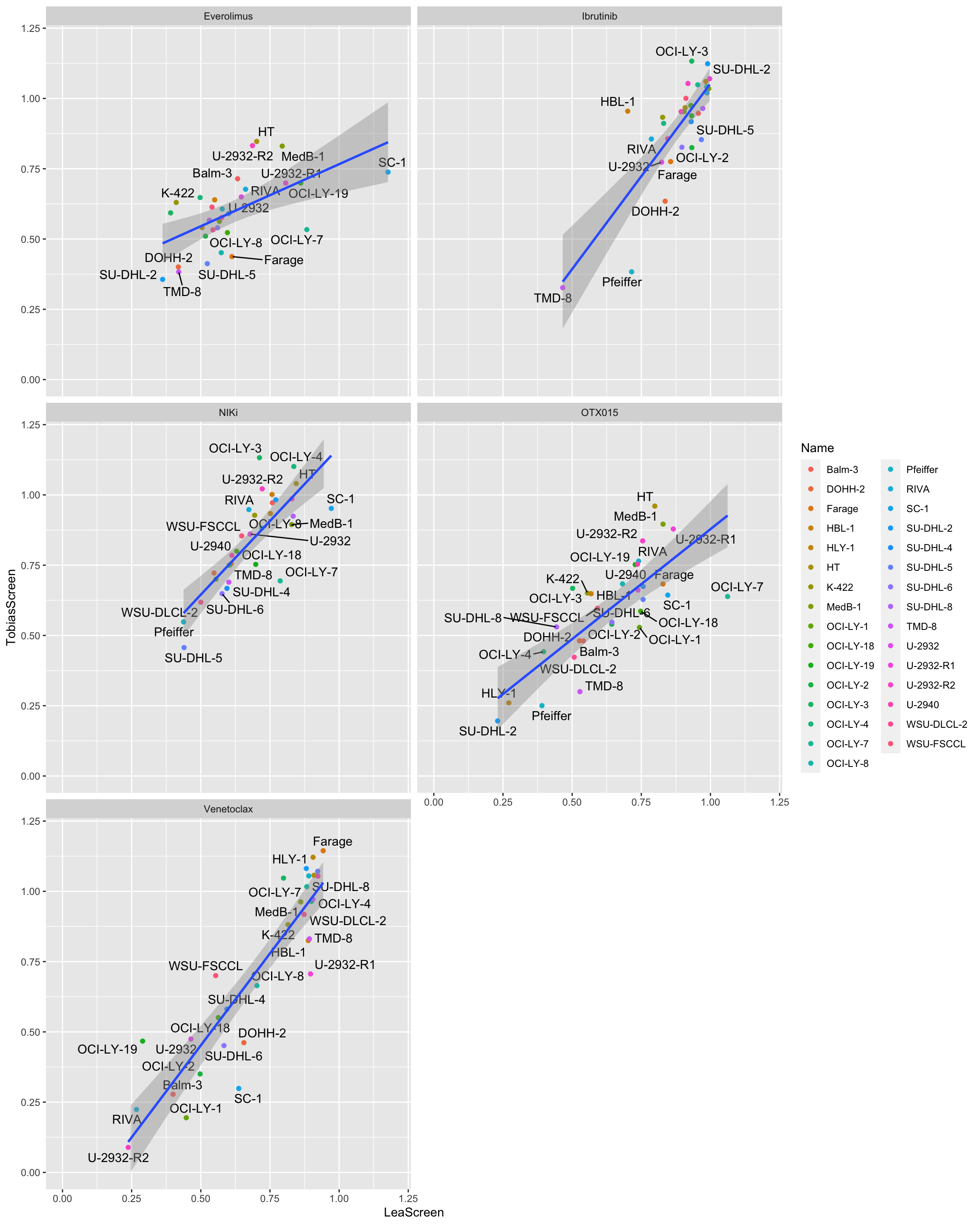
Compare the Doxorubicine results from Lea’s main screen and that from Tobias screen
load("../data/CHOP_screen_all_data.RData")

pilotTab <- CHOP_Screen_data %>%
  filter(drug == "Doxorubicin") %>%
  group_by(Name, Drug_Conc, drug) %>%
  summarise(normVal = mean(Normalized_values)) %>%
  dplyr::rename(Drug = drug, conc = Drug_Conc) %>%
  mutate(conc =as.numeric(conc), Name = str_replace_all(Name, "_", "-"))
`summarise()` has grouped output by 'Name', 'Drug_Conc'. You can override using
the `.groups` argument. aucTab <- pilotTab %>% group_by(Name, Drug) %>%
summarise(auc = calcAUC(normVal, conc))`summarise()` has grouped output by 'Name'. You can override using the
`.groups` argument.pilotTab <- pilotTab %>% left_join(aucTab) %>%
mutate(screen = "pilotScreen") %>%
ungroup()Joining, by = c("Name", "Drug")Process the old screen data by Tobias
doxoTab <- filter(Screen.CL19, Drug %in% "Doxorubicine", Name %in% pilotTab$Name, TimePoint == "48 h") %>%
  dplyr::rename(normVal = Normalized, conc = Drug.Conc) %>%
  group_by(Name, Drug, conc) %>%
  summarise(normVal = mean(normVal, na.rm=TRUE))
`summarise()` has grouped output by 'Name', 'Drug'. You can override using the
`.groups` argument.aucTab <- doxoTab %>% group_by(Name, Drug) %>%
summarise(auc = calcAUC(normVal, conc))`summarise()` has grouped output by 'Name'. You can override using the
`.groups` argument.doxoTab <- doxoTab %>% left_join(aucTab) %>%
mutate(screen = "screenTobias")Joining, by = c("Name", "Drug")Dose-response curves
comTab <- bind_rows(pilotTab, doxoTab)
ggplot(comTab, aes(x=conc, y=normVal, col=screen)) +
  geom_point() + geom_line() +
  facet_wrap(~Name, ncol=4) +
  scale_x_log10() +
  ylim(0,1.6)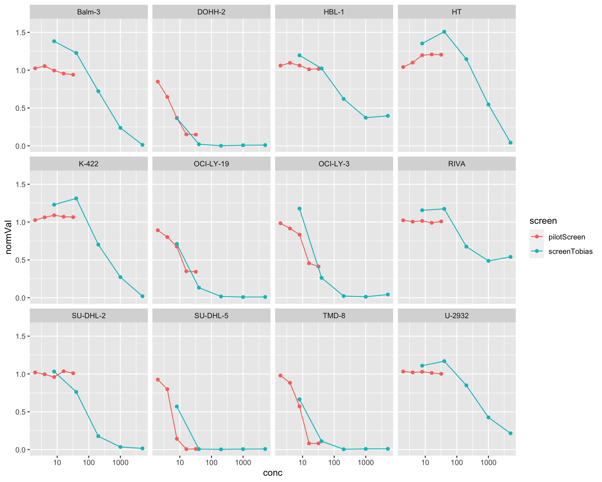
AUC correlation
plotTab <- distinct(comTab, Name, auc, screen) %>%
  pivot_wider(names_from = screen, values_from = auc) %>%
  left_join(tp53Tab)
Joining, by = "Name"ggplot(plotTab, aes(x=pilotScreen, y=screenTobias)) +
geom_point(aes(col = TP53)) +
ggrepel::geom_text_repel(aes(label = Name)) +
geom_smooth(method = "lm") +
xlim(0,1.5) + ylim(0,1.5) +
geom_abline(intercept = 0, slope = 1, color = "red", lintype = "dotted")Warning: Ignoring unknown parameters: lintype`geom_smooth()` using formula 'y ~ x'Warning: Removed 5 rows containing missing values (geom_smooth).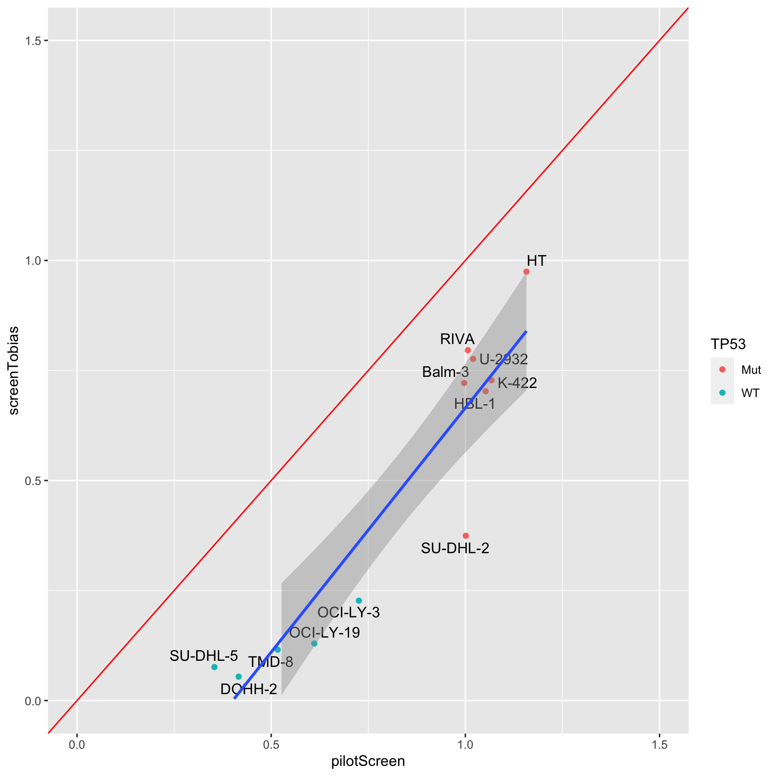
Define a sensitive-resistant table based on pilot screen
clusterTab <- distinct(pilotTab, Name, auc) %>%
  mutate(cluster = ifelse(auc > 0.75, "resistant","sensitive")) %>%
  select(-auc)
Compare the CHP result from Lea’s main screen and the Doxorubicine results from Tobias screen
Process the new screen data by Lea
chpTab <- filter(screenData, Drug_A %in% "DMSO", Name %in% overCell, Drug_B == "CHP", Plate == "CHP:Pola") %>%
  group_by(Name, Drug_B, Drug_B.Conc) %>%
  summarise(normVal = mean(normVal, na.rm=TRUE)) %>%
  rename(Drug = Drug_B, conc = Drug_B.Conc)
`summarise()` has grouped output by 'Name', 'Drug_B'. You can override using
the `.groups` argument.aucTab <- chpTab %>% group_by(Name, Drug) %>%
summarise(auc = calcAUC(normVal, conc))`summarise()` has grouped output by 'Name'. You can override using the
`.groups` argument.chpTab <- chpTab %>% left_join(aucTab) %>%
mutate(screen = "CHP")Joining, by = c("Name", "Drug")Process the old screen data by Tobias
doxoTab <- filter(Screen.CL19, Drug %in% "Doxorubicine", Name %in% overCell, TimePoint == "48 h") %>%
  dplyr::rename(normVal = Normalized, conc = Drug.Conc) %>%
  group_by(Name, Drug, conc) %>%
  summarise(normVal = mean(normVal, na.rm=TRUE))
`summarise()` has grouped output by 'Name', 'Drug'. You can override using the
`.groups` argument.aucTab <- doxoTab %>% group_by(Name, Drug) %>%
summarise(auc = calcAUC(normVal, conc))`summarise()` has grouped output by 'Name'. You can override using the
`.groups` argument.doxoTab <- doxoTab %>% left_join(aucTab) %>%
mutate(screen = "Doxorubicin")Joining, by = c("Name", "Drug")Dose-response curves
comTab <- bind_rows(chpTab, doxoTab)
ggplot(comTab, aes(x=conc, y=normVal, col=screen)) +
  geom_point() + geom_line() +
  facet_wrap(~Name, ncol=4) +
  scale_x_log10() +
  ylim(0,1.6)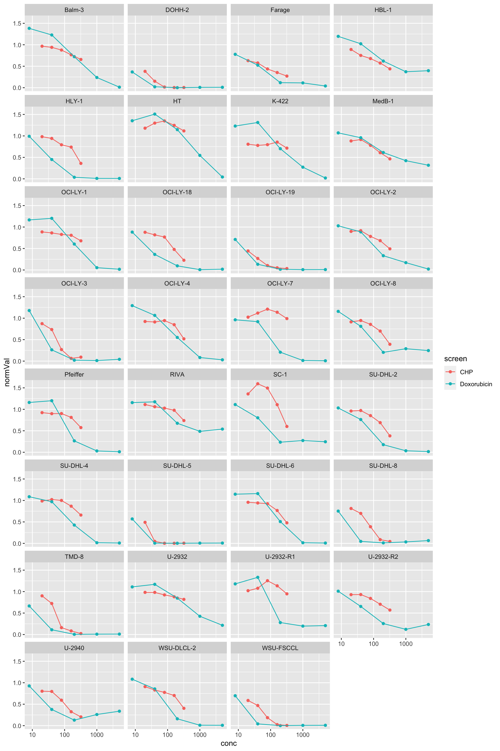
AUC correlation
Color by TP53 mutation
plotTab <- distinct(comTab, Name, auc, Drug) %>%
  pivot_wider(names_from = Drug, values_from = auc) %>%
  left_join(tp53Tab) %>%
  left_join(clusterTab) %>%
  mutate(TP53=replace_na(TP53, "unknown"),
         cluster = replace_na(cluster, "undefined"))
Joining, by = "Name"
Joining, by = "Name"ggplot(plotTab, aes(x=CHP, y=Doxorubicine)) +
geom_point(aes(col = TP53)) +
ggrepel::geom_text_repel(aes(label = Name)) +
geom_smooth(method = "lm") +
xlim(0,1.5) + ylim(0,1.5) +
geom_abline(intercept = 0, slope = 1, color = "red", lintype = "dotted")Warning: Ignoring unknown parameters: lintype`geom_smooth()` using formula 'y ~ x'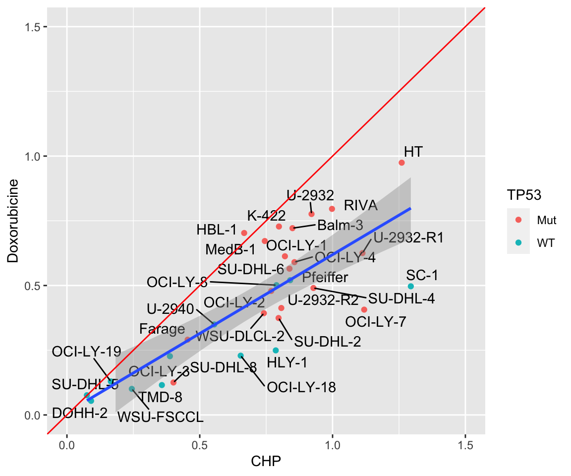 Color by resistant cluster defined by pilot screen
ggplot(plotTab, aes(x=CHP, y=Doxorubicine)) +
  geom_point(aes(col = cluster)) +
  ggrepel::geom_text_repel(aes(label = Name)) +
  geom_smooth(method = "lm") +
  xlim(0,1.5) + ylim(0,1.5) +
  geom_abline(intercept = 0, slope = 1, color = "red", lintype = "dotted")
Warning: Ignoring unknown parameters: lintype`geom_smooth()` using formula 'y ~ x'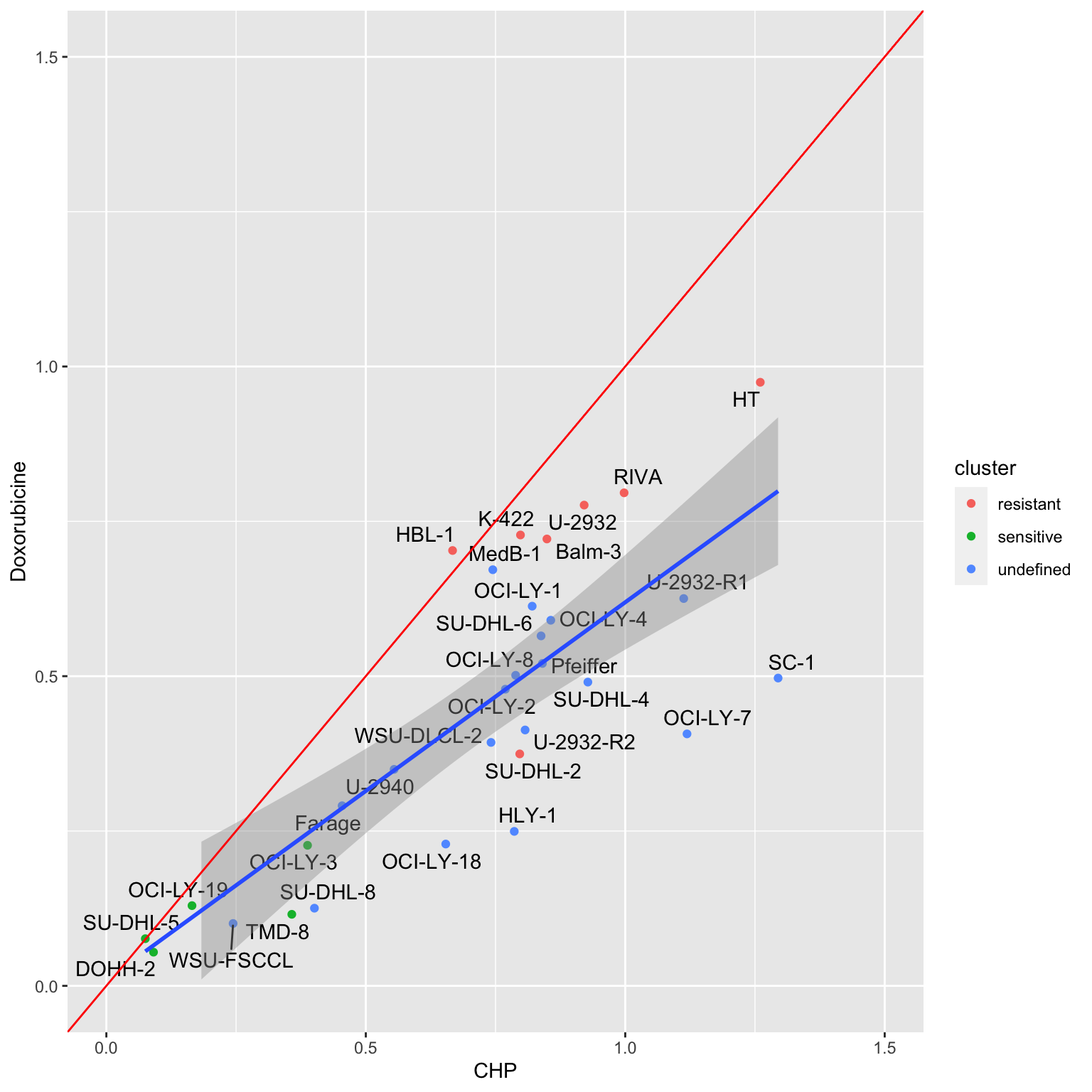
sessionInfo()R version 4.2.0 (2022-04-22)
Platform: x86_64-apple-darwin17.0 (64-bit)
Running under: macOS Big Sur/Monterey 10.16
Matrix products: default
BLAS: /Library/Frameworks/R.framework/Versions/4.2/Resources/lib/libRblas.0.dylib
LAPACK: /Library/Frameworks/R.framework/Versions/4.2/Resources/lib/libRlapack.dylib
locale:
[1] en_US.UTF-8/en_US.UTF-8/en_US.UTF-8/C/en_US.UTF-8/en_US.UTF-8
attached base packages:
[1] stats graphics grDevices utils datasets methods base
other attached packages:
[1] gridExtra_2.3 forcats_0.5.1 stringr_1.4.1 dplyr_1.0.9
[5] purrr_0.3.4 readr_2.1.2 tidyr_1.2.0 tibble_3.1.8
[9] ggplot2_3.3.6 tidyverse_1.3.2
loaded via a namespace (and not attached):
[1] readxl_1.4.0 backports_1.4.1
[3] fastmatch_1.1-3 drc_3.0-1
[5] jyluMisc_0.1.5 workflowr_1.7.0
[7] igraph_1.3.4 shinydashboard_0.7.2
[9] splines_4.2.0 crosstalk_1.2.0
[11] BiocParallel_1.30.3 GenomeInfoDb_1.32.2
[13] TH.data_1.1-1 digest_0.6.30
[15] htmltools_0.5.3 fansi_1.0.3
[17] magrittr_2.0.3 googlesheets4_1.0.0
[19] cluster_2.1.3 tzdb_0.3.0
[21] limma_3.52.2 modelr_0.1.8
[23] matrixStats_0.62.0 sandwich_3.0-2
[25] piano_2.12.0 colorspace_2.0-3
[27] ggrepel_0.9.1 rvest_1.0.2
[29] haven_2.5.0 xfun_0.31
[31] crayon_1.5.2 RCurl_1.98-1.7
[33] jsonlite_1.8.3 survival_3.4-0
[35] zoo_1.8-10 glue_1.6.2
[37] survminer_0.4.9 gtable_0.3.0
[39] gargle_1.2.0 zlibbioc_1.42.0
[41] XVector_0.36.0 DelayedArray_0.22.0
[43] car_3.1-0 BiocGenerics_0.42.0
[45] abind_1.4-5 scales_1.2.0
[47] mvtnorm_1.1-3 DBI_1.1.3
[49] relations_0.6-12 rstatix_0.7.0
[51] Rcpp_1.0.9 plotrix_3.8-2
[53] xtable_1.8-4 km.ci_0.5-6
[55] stats4_4.2.0 DT_0.23
[57] htmlwidgets_1.5.4 httr_1.4.3
[59] fgsea_1.22.0 gplots_3.1.3
[61] ellipsis_0.3.2 pkgconfig_2.0.3
[63] farver_2.1.1 sass_0.4.2
[65] dbplyr_2.2.1 utf8_1.2.2
[67] labeling_0.4.2 tidyselect_1.1.2
[69] rlang_1.0.6 later_1.3.0
[71] munsell_0.5.0 cellranger_1.1.0
[73] tools_4.2.0 visNetwork_2.1.0
[75] cachem_1.0.6 cli_3.4.1
[77] generics_0.1.3 broom_1.0.0
[79] evaluate_0.15 fastmap_1.1.0
[81] yaml_2.3.5 knitr_1.39
[83] fs_1.5.2 survMisc_0.5.6
[85] caTools_1.18.2 nlme_3.1-158
[87] mime_0.12 slam_0.1-50
[89] xml2_1.3.3 compiler_4.2.0
[91] rstudioapi_0.13 beeswarm_0.4.0
[93] ggsignif_0.6.3 marray_1.74.0
[95] reprex_2.0.1 bslib_0.4.1
[97] stringi_1.7.8 highr_0.9
[99] lattice_0.20-45 Matrix_1.4-1
[101] KMsurv_0.1-5 shinyjs_2.1.0
[103] vctrs_0.4.1 pillar_1.8.0
[105] lifecycle_1.0.3 jquerylib_0.1.4
[107] data.table_1.14.2 cowplot_1.1.1
[109] bitops_1.0-7 httpuv_1.6.6
[111] GenomicRanges_1.48.0 R6_2.5.1
[113] promises_1.2.0.1 KernSmooth_2.23-20
[115] vipor_0.4.5 IRanges_2.30.0
[117] codetools_0.2-18 MASS_7.3-58
[119] gtools_3.9.3 exactRankTests_0.8-35
[121] assertthat_0.2.1 SummarizedExperiment_1.26.1
[123] rprojroot_2.0.3 withr_2.5.0
[125] multcomp_1.4-19 S4Vectors_0.34.0
[127] GenomeInfoDbData_1.2.8 mgcv_1.8-40
[129] parallel_4.2.0 hms_1.1.1
[131] grid_4.2.0 rmarkdown_2.14
[133] MatrixGenerics_1.8.1 carData_3.0-5
[135] googledrive_2.0.0 ggpubr_0.4.0
[137] git2r_0.30.1 maxstat_0.7-25
[139] sets_1.0-21 Biobase_2.56.0
[141] shiny_1.7.3 lubridate_1.8.0
[143] ggbeeswarm_0.6.0