Analysis focused on the single agent effect
Junyan Lu
2022-04-25
Last updated: 2022-07-08
Checks: 5 1
Knit directory: combiDLBCL/analysis/
This reproducible R Markdown analysis was created with workflowr (version 1.7.0). The Checks tab describes the reproducibility checks that were applied when the results were created. The Past versions tab lists the development history.
Great job! The global environment was empty. Objects defined in the global environment can affect the analysis in your R Markdown file in unknown ways. For reproduciblity it’s best to always run the code in an empty environment.
The command set.seed(20220425) was run prior to running
the code in the R Markdown file. Setting a seed ensures that any results
that rely on randomness, e.g. subsampling or permutations, are
reproducible.
Great job! Recording the operating system, R version, and package versions is critical for reproducibility.
Nice! There were no cached chunks for this analysis, so you can be confident that you successfully produced the results during this run.
Great job! Using relative paths to the files within your workflowr project makes it easier to run your code on other machines.
Tracking code development and connecting the code version to the
results is critical for reproducibility. To start using Git, open the
Terminal and type git init in your project directory.
This project is not being versioned with Git. To obtain the full
reproducibility benefits of using workflowr, please see
?wflow_start.
Load libraries and datasets
Data preprocessing
Drug screen data
Subset for Pola plates
screenData <- filter(screenData, Plate =="CHP:Pola")Get combi-drug
singleViab <- filter(screenData, Drug_B.Conc ==0, Drug_A.Conc!=0) %>%
  mutate(Drug = Drug_A, Conc = Drug_A.Conc, ConcStep = Drug_A.ConcStep) %>%
  select(Name, Drug, Conc, ConcStep, normVal)
Get base-drug
baseViab <- filter(screenData, Drug_A.Conc ==0, Drug_B.Conc!=0) %>%
  mutate(Drug = Drug_B, Conc = Drug_B.Conc, ConcStep = Drug_B.ConcStep) %>%
  select(Name, Drug, Conc, ConcStep, normVal)
Combine and summarise
viabTab.conc <- bind_rows(singleViab, baseViab) #individual concentration
viabTab <- group_by(viabTab.conc, Name, Drug) %>%
  summarise(viab = calcAUC(normVal, Conc)) %>%
  ungroup()
`summarise()` has grouped output by 'Name'. You can override using the
`.groups` argument.Genomic data
SNVs
load("../data/SVs.RData")Define meaningful mutations Only choose mutation not on IG genes and have cosmic annotation (either old or new)
muts <- c("frameshift deletion", "frameshift insertion",
          "nonsynonymous","stopgain","stoploss")
svTab <- filter(SVs, Classification %in% muts,
                !str_detect(Gene,"IG[HKL][VDJ]"),
                Cosmic_old %in% "Yes" | !is.na(Cosmic_new))
Filter for known cancer genes in DLBCL (Chapuy et al., 2018)
pubGene <- readxl::read_xlsx("../data/41591_2018_16_MOESM5_ESM.xlsx", sheet = 1, skip = 1) %>%
  filter(q<0.1)
New names:
• `` -> `...19`
• `` -> `...20`
• `` -> `...22`svTab <- filter(svTab, Gene %in% pubGene$gene)How many cell lines have genomic information
table(unique(viabTab$Name) %in% svTab$Name)
FALSE  TRUE
    1    31
Save the filtered table
save(svTab, file = "../data/SVs_filtered.RData")Summarise mutations (cell lines used in drug screen): count as gene mutation if there is at least one mutation within gene
mutTab <- group_by(svTab, Name, Gene) %>% summarise(n = length(Name)) %>%
  arrange(desc(n)) %>%
  filter(Name %in% viabTab$Name)
`summarise()` has grouped output by 'Name'. You can override using the
`.groups` argument.#Get mutations occured at least in three cell lines
geneCount <- group_by(mutTab, Gene) %>% summarise(n=length(Name)) %>%
filter(n>=3) %>% arrange(desc(n)) %>%
mutate(Gene = factor(Gene, levels = Gene))There are too many mutations. Manual curation maybe needed.
Occurrence of mutations among cell lines, only mutations occurred at least 3 times are considered
ggplot(geneCount, aes(x=Gene, y=n)) +
  geom_bar(stat = "identity") +
  theme_bw() + theme(axis.text.x = element_text(angle = 90, hjust = 1, vjust = 0.5))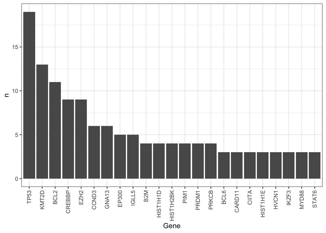
Summarise plot of genomics
Only use mutations that occurred at least five time in all the cell lines
mutTabSub <- filter(mutTab, Gene %in% geneCount$Gene) %>%
  mutate(status =1) %>% select(Name, Gene, status) %>%
  pivot_wider(names_from = "Gene", values_from = "status") %>%
  mutate_all(replace_na,0) %>%
  pivot_longer(-Name, names_to = "Gene", values_to = "status")
`mutate_all()` ignored the following grouping variables:
• Column `Name`
ℹ Use `mutate_at(df, vars(-group_cols()), myoperation)` to silence the message.geneMat <- mutTabSub %>% pivot_wider(names_from = "Gene", values_from = "status") %>%
column_to_rownames("Name") %>% as.matrix()
geneMat <- geneMat[,order(colSums(geneMat))]Prepare plot
sortTab <- function(sumTab) {
  i <- ncol(sumTab)
  #print(i)
  if (i == 1) {
    return(rownames(sumTab)[order(sumTab[,i])])
  }
  allLevel <- sort(unique(sumTab[,i]))
  orderRow <- lapply(allLevel, function(n) {
    sortTab(sumTab[sumTab[,i] %in% n, seq(1,i-1), drop = FALSE])
  }) %>% unlist() %>% c()
  return(orderRow)
}

sortedPat <- rev(sortTab(geneMat))
plotTab <- mutTabSub %>% mutate(Name = factor(Name, levels = sortedPat),
Gene = factor(Gene, levels = colnames(geneMat)))
ggplot(plotTab, aes(x=Name, y=Gene)) +
geom_tile(aes(fill = factor(status)), col = "grey50") +
scale_fill_manual(values = c(`1`="black",`0`="white"), name = "mutation") +
theme(axis.text.x = element_text(angle = 90, hjust=1, vjust=0.5)) 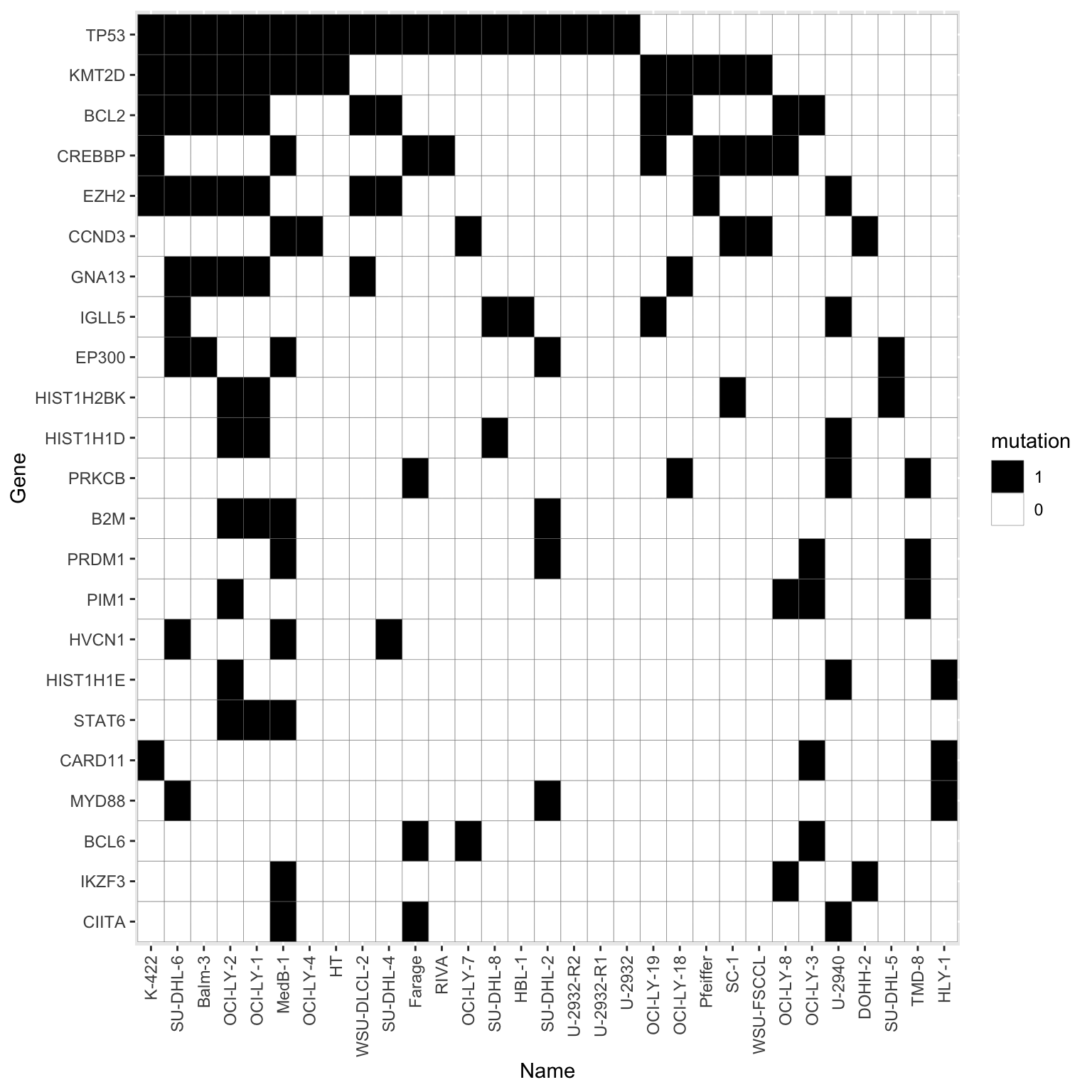
CNVs
load("../data/CNVs.RData")
cnvTab <- CNVs %>% mutate(change = case_when(
  cn == 2 ~ "normal",
  cn > 2 ~ "gain",
  cn < 2 ~ "del"
)) %>%
  filter(change != "normal", gene!="-") %>%
  mutate(cnv = paste0(gene,"_",change))

cnvTab <- distinct(cnvTab, cnv, gene, Name) %>%
  mutate(Gene = cnv) %>%
  select(Name, Gene)

#save a table
save(cnvTab, file = "../data/CNVs_filtered.RData")
Summarise mutations (cell lines used in drug screen): count as gene mutation if there is at least one mutation within gene
cnTab <- cnvTab %>%
  filter(Name %in% viabTab$Name)

#Get mutations occured at least in three cell lines
geneCount <- group_by(cnTab, Gene) %>% summarise(n=length(Name)) %>%
  filter(n>=3) %>% arrange(desc(n)) %>%
  mutate(Gene = factor(Gene, levels = Gene))
There are too many mutations. Manual curation maybe needed.
Occurrence of mutations among cell lines, only mutations occurred at least 3 times are considered
ggplot(geneCount, aes(x=Gene, y=n)) +
  geom_bar(stat = "identity") +
  theme_bw() + theme(axis.text.x = element_text(angle = 90, hjust = 1, vjust = 0.5))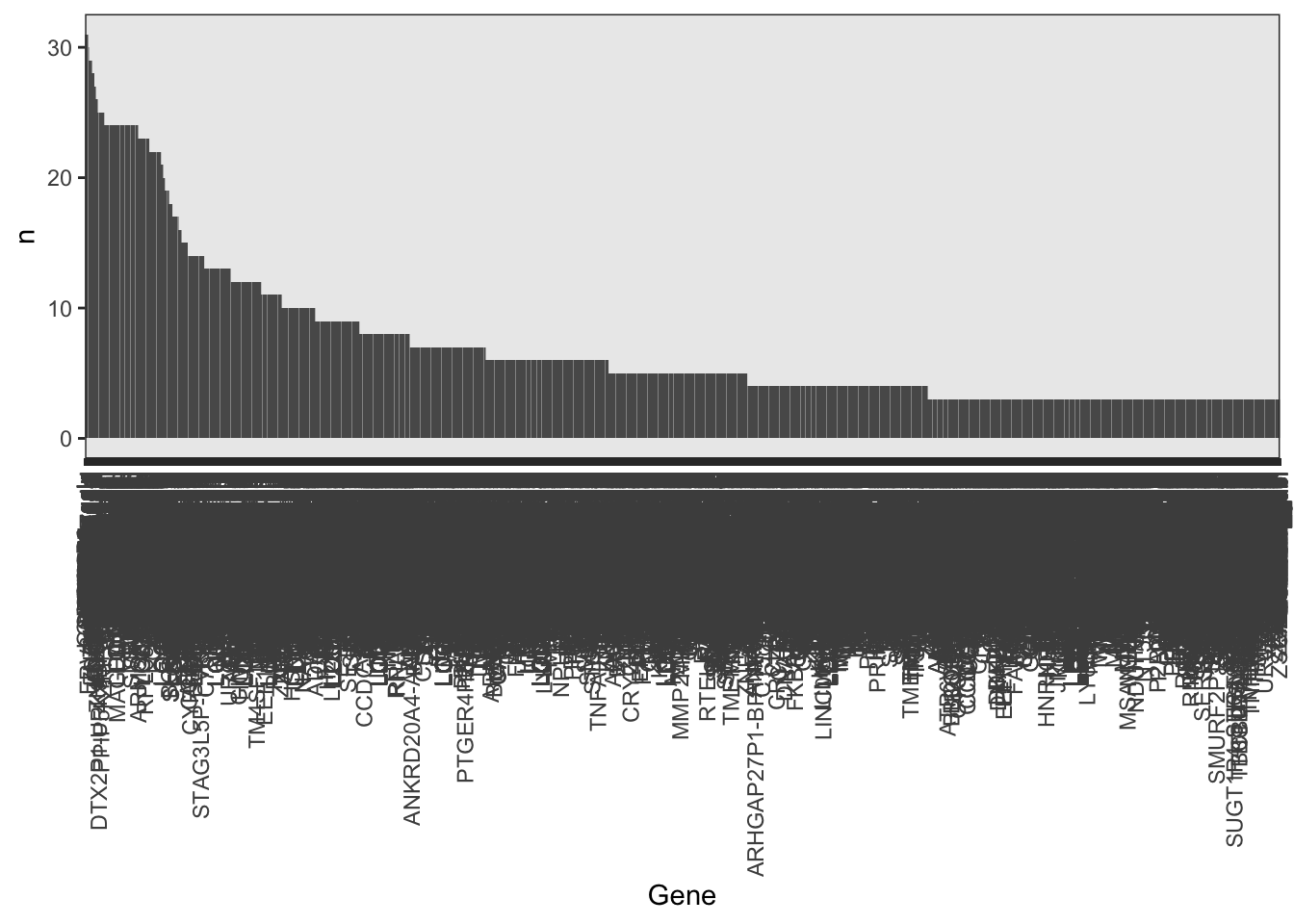
Exploratory data analysis
Hierarchical clustering visualization
library(pheatmap)

viabMat <- viabTab %>% pivot_wider(names_from = Name, values_from = viab) %>%
  column_to_rownames("Drug") %>% as.matrix()

atpCount <- filter(screenData, Drug_A.Conc ==0, Drug_B.Conc ==0, !ifEdge) %>%
  group_by(Name) %>% summarise(atp = median(Count)) %>%
  mutate(logATP = log2(atp))

seleGenes <- c("TP53","EZH2","MYC","FOXO1","EP300","CACNA1E","BCL2")

colAnno <- tibble(Name = colnames(viabMat)) %>%
  left_join(mutTabSub,by="Name") %>% filter(Gene %in% seleGenes) %>%
  pivot_wider(names_from = "Gene", values_from = "status") %>%
  mutate(baseATP = atpCount[match(Name, atpCount$Name),]$logATP) %>%
  data.frame() %>% column_to_rownames("Name")

pheatmap(viabMat, scale = "row", clustering_method = "ward.D2", annotation_col = colAnno)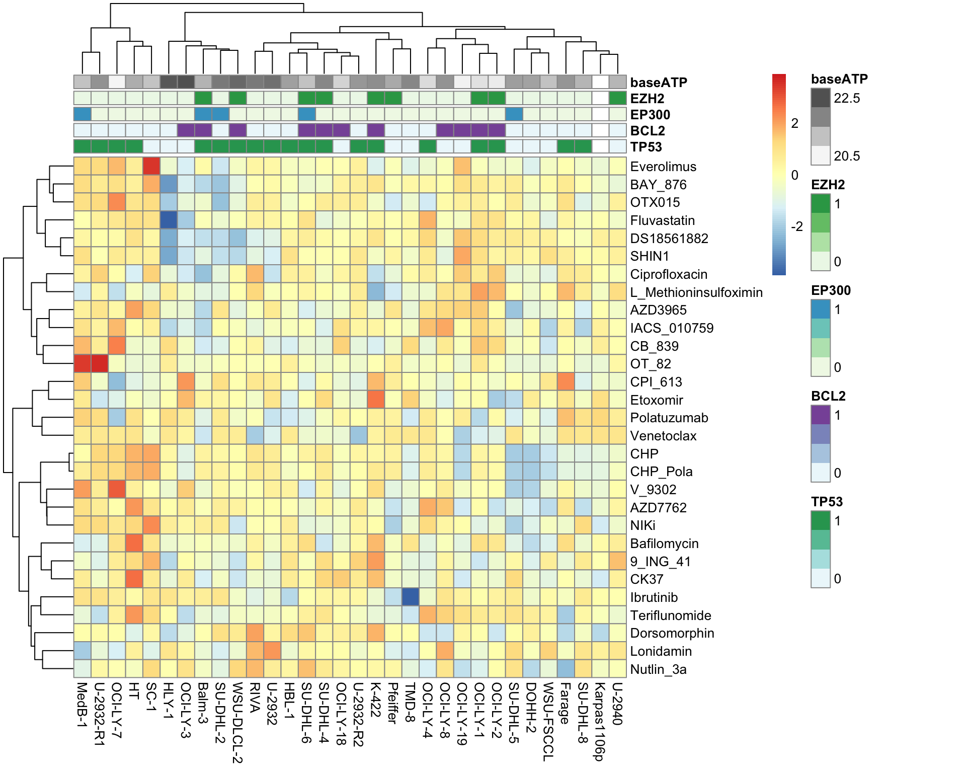
PCA
Calculate PCA
pcRes <- prcomp(t(viabMat), scale. = FALSE, center = TRUE)
pcTab <- pcRes$x[,1:10] %>% as_tibble(rownames = "Name")
varExp <- (pcRes$sdev^2)/sum(pcRes$sdev^2)
Plot PC1 and PC2
ggplot(pcTab, aes(x=PC1, y=PC2, label = Name, col=Name)) +
  xlab(sprintf("PC1 (%1.1f%%)", 100*varExp[1])) + ylab(sprintf("PC2 (%1.1f%%)", 100*varExp[2])) +
  geom_point() +
  ggrepel::geom_text_repel() +
  theme(legend.position = "none")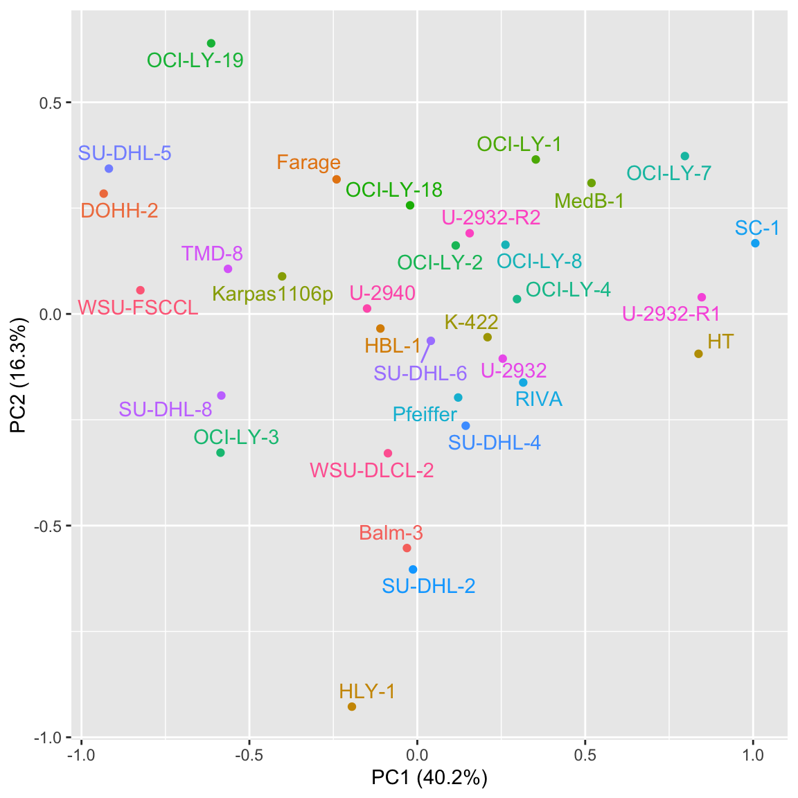
Correlate top10 PCs with baseline ATP count
testTab <- pcTab %>% pivot_longer(-Name, names_to = "PC", values_to = "value") %>%
  left_join(atpCount, by = "Name")

resTab <- group_by(testTab, PC) %>% nest() %>%
  mutate(m=map(data, ~cor.test(~value+logATP,.))) %>%
  mutate(res=map(m, broom::tidy)) %>% unnest(res) %>%
  arrange(p.value) %>%
  select(PC, estimate, p.value)
head(resTab)
# A tibble: 6 × 3
# Groups: PC [6]
PC estimate p.value
<chr> <dbl> <dbl>
1 PC2 -0.651 0.0000552
2 PC10 -0.256 0.157
3 PC1 -0.191 0.295
4 PC9 -0.170 0.354
5 PC3 0.158 0.389
6 PC8 0.143 0.435 PC2 is potentially associated with baseline ATP level
plotTab <- pcTab %>% left_join(atpCount, by ="Name")
ggplot(plotTab, aes(x=PC1, y=PC2, label = Name, col=logATP)) +
  xlab(sprintf("PC1 (%1.1f%%)", 100*varExp[1])) + ylab(sprintf("PC2 (%1.1f%%)", 100*varExp[2])) +
  geom_point() +
  scale_color_gradient(low = "blue",high = "red") +
ggrepel::geom_text_repel() 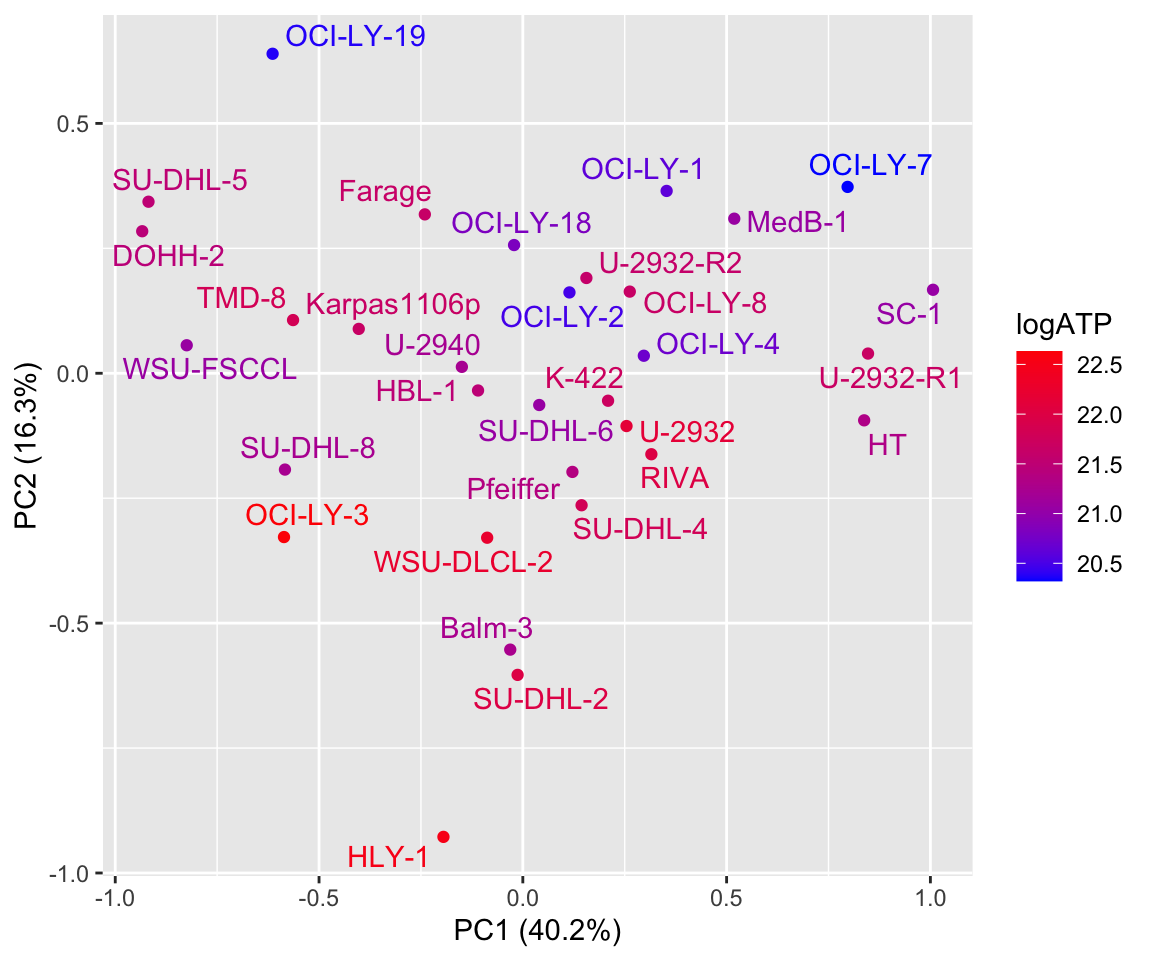
Correlate top10 PCs with genomic background
testTab <- pcTab %>% pivot_longer(-Name, names_to = "PC", values_to = "value") %>%
  full_join(mutTabSub, by = "Name") %>%
  filter(!is.na(status))

resTab <- group_by(testTab, PC, Gene) %>% nest() %>%
  mutate(m=map(data, ~t.test(value~status,.,var.equal=TRUE))) %>%
  mutate(res=map(m, broom::tidy)) %>% unnest(res) %>%
  arrange(p.value) %>%
  select(PC, estimate, p.value) %>%
  ungroup() %>%
  mutate(p.adj = p.adjust(p.value, method = "BH"))
Adding missing grouping variables: `Gene`head(resTab)# A tibble: 6 × 5
Gene PC estimate p.value p.adj
<chr> <chr> <dbl> <dbl> <dbl>
1 MYD88 PC2 0.585 0.00185 0.423
2 EZH2 PC10 -0.0980 0.00467 0.423
3 TP53 PC1 -0.486 0.00744 0.423
4 CIITA PC3 -0.435 0.00854 0.423
5 BCL6 PC7 -0.225 0.00946 0.423
6 EZH2 PC6 0.156 0.0114 0.423P-value histogram
hist(resTab$p.value)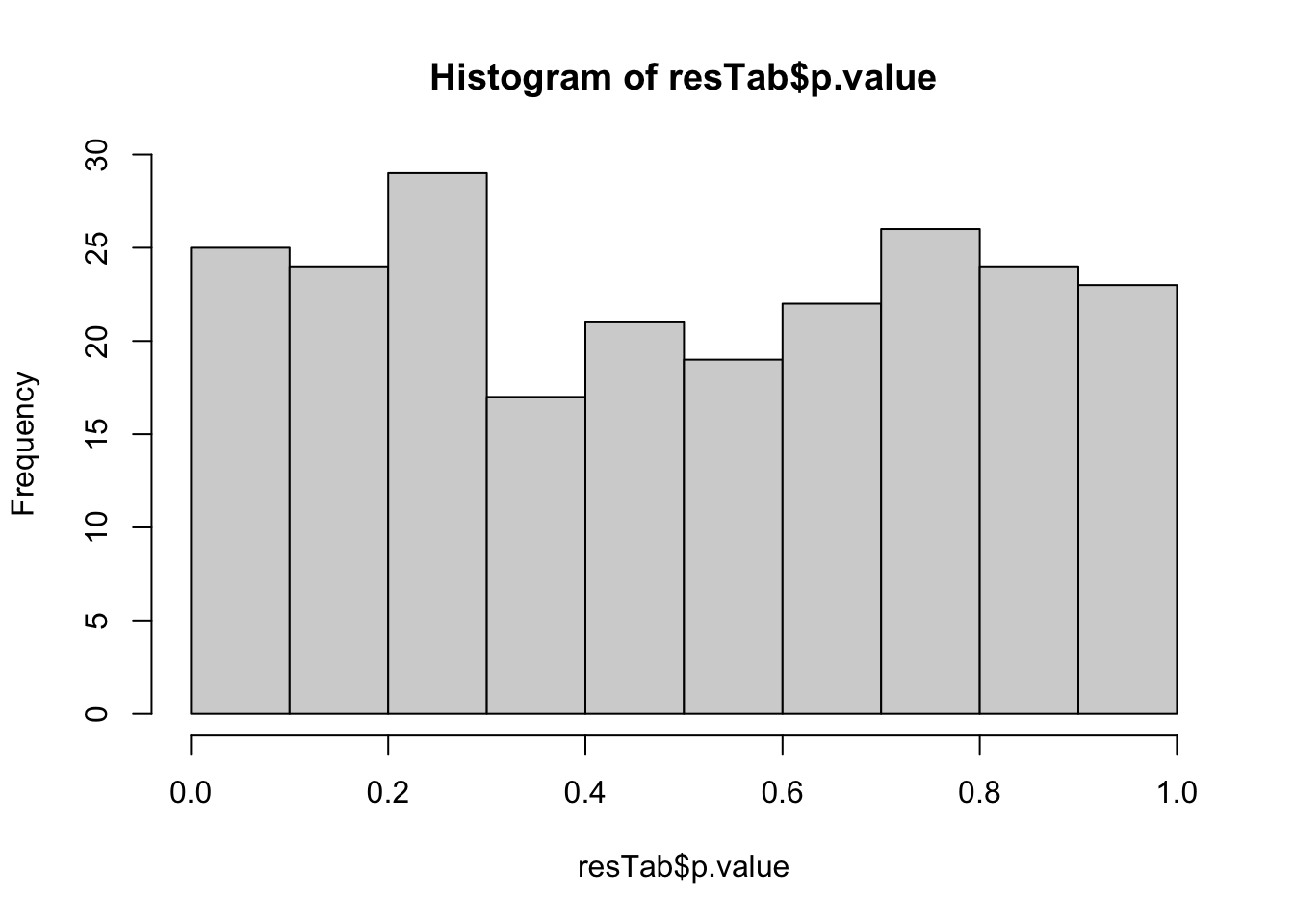 TP53 may associate with PC1
plotTab <- mutate(plotTab, TP53 = factor(colAnno[Name,]$TP53))
ggplot(plotTab, aes(x=PC1, y=PC2, label = Name, col=TP53)) +
  xlab(sprintf("PC1 (%1.1f%%)", 100*varExp[1])) + ylab(sprintf("PC2 (%1.1f%%)", 100*varExp[2])) +
  geom_point() +
  #scale_color_gradient(low = "blue",high = "red") +
  ggrepel::geom_text_repel() +
  theme_bw()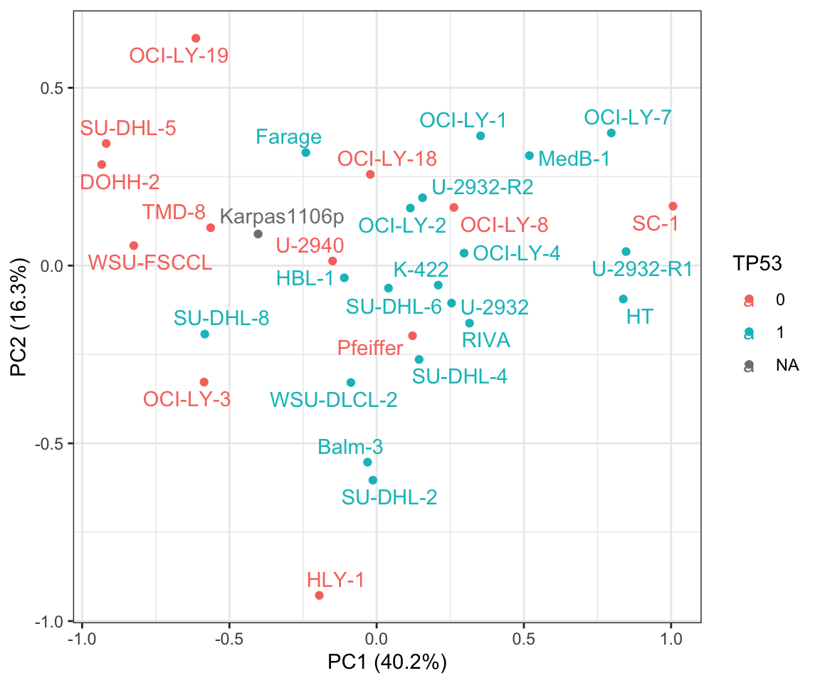
Association between drug responses and genomics
Perform t-test
testTab <- full_join(viabTab, mutTabSub, by = "Name") %>%
  filter(!is.na(status))
resTab <- group_by(testTab, Drug, Gene) %>% nest() %>%
  mutate(m = map(data, ~t.test(viab ~ status, ., var.equal=TRUE))) %>%
  mutate(res = map(m, broom::tidy)) %>%
  unnest(res) %>%
  select(Drug, Gene, p.value) %>%
  arrange(p.value) %>%
  ungroup() %>%
  mutate(p.adj = p.adjust(p.value, method="BH"))
P-value histogram
hist(resTab$p.value)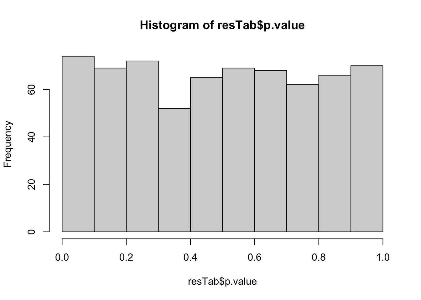 All results with P<0.01
resTab.sig <- filter(resTab, p.value < 0.01)
resTab.sig %>% mutate_if(is.numeric, formatC, digits=1) %>% DT::datatable()
No one passed 10% FDR, probably too many test
Boxplot of significant pairs (0.01)
pList <- lapply(seq(nrow(resTab.sig)), function(i) {
  rec <- resTab.sig[i,]
  plotTab <- filter(testTab, Drug == rec$Drug, Gene == rec$Gene) %>%
    mutate(status = ifelse(status ==1, "Mut","WT"))
  ggplot(plotTab, aes(x=status, y=viab)) +
    geom_boxplot(outlier.shape = NA) +
    ggbeeswarm::geom_quasirandom(aes(col = status)) +
    theme_bw() +
    theme(legend.position = "none") +
    ggtitle(sprintf("%s ~ %s (p=%s)", rec$Drug, rec$Gene, formatC(rec$p.value, digits=2, format="e")))
})
cowplot::plot_grid(plotlist=pList,ncol=3)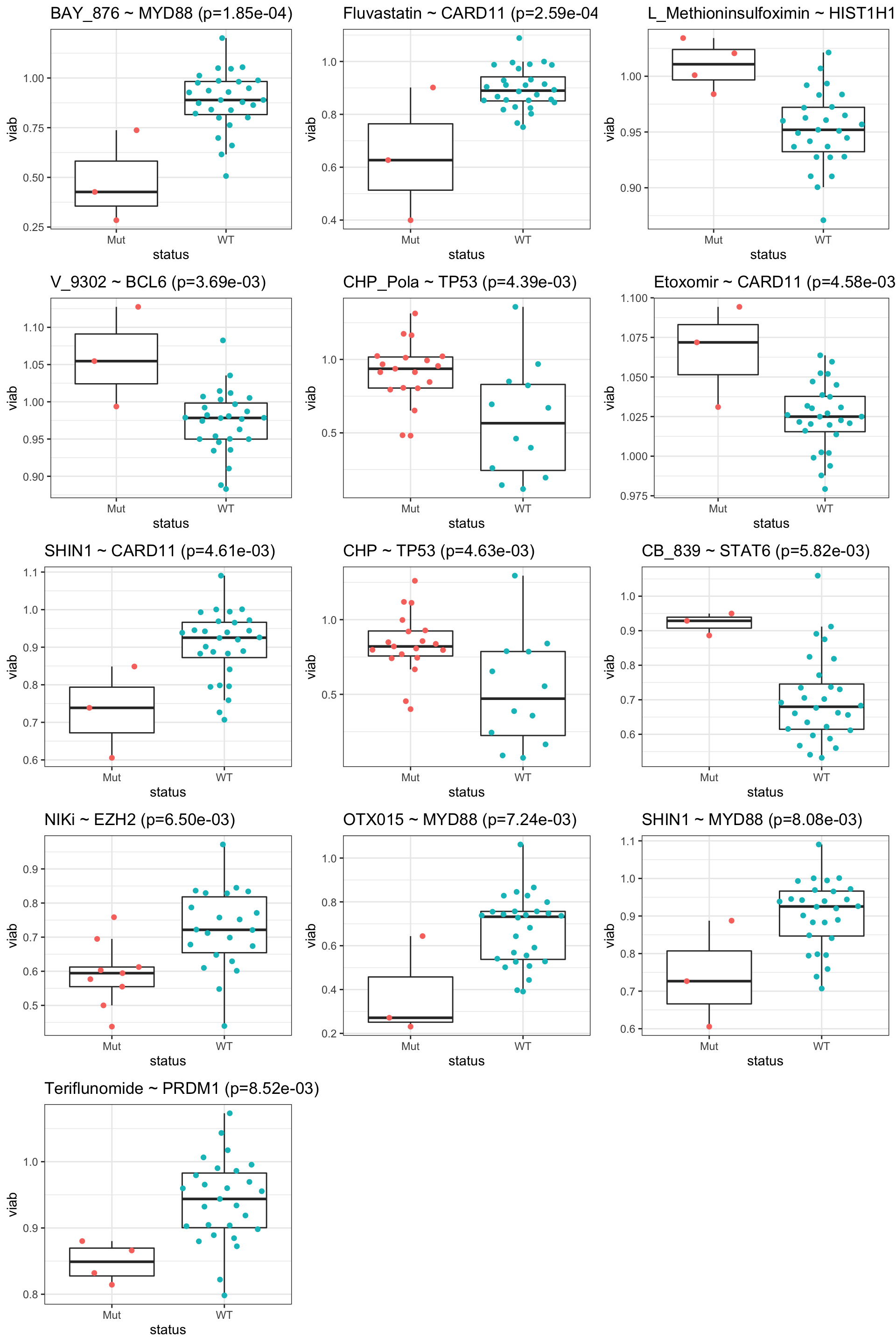
Consensus clustering analysis
Run clustering with ConcsensusClustterPlus
library(ConsensusClusterPlus)
#consensus clustering
#Center each feature by median
d <- sweep(viabMat,1, apply(viabMat,1, median, na.rm=T))

resConsClust <- ConsensusClusterPlus(viabMat, maxK=10, reps=1000 , pItem=0.8, pFeature=0.8, title = "DLBCL_conc",
                            clusterAlg="hc",distance="pearson",
                            seed=2022, plot="png")
end fractionclustered
clustered
clustered
clustered
clustered
clustered
clustered
clustered
clustered#plot clustering result
icl = calcICL(resConsClust,title="DLBCL_conc",plot="png")
#save results for later use
#save(resConsClust, file = "../output/resConsClust.RData")Based on delta curve, three clusters would be most appropriate
Post-processing consensus clustering results
Select samples with clustering consensus over 80%
k=5
conMat <- resConsClust[[k]]$consensusMatrix
conClust <- resConsClust[[k]]$consensusClass
colnames(conMat) <- colnames(viabMat)
Visualization
geneAnno <- mutTabSub %>% filter(Gene %in% seleGenes) %>%
  pivot_wider(names_from = "Gene", values_from = "status")
colAnno <- tibble(Name = colnames(viabMat),
                  Cluster = factor(conClust)) %>%
  left_join(geneAnno, by ="Name") %>%
  mutate(baseATP = atpCount[match(Name, atpCount$Name),]$logATP) %>%
  data.frame() %>% column_to_rownames("Name")

pheatmap(conMat, annotation_col = colAnno, method = "complete", clustering_distance_rows = "correlation", clustering_distance_cols = "correlation")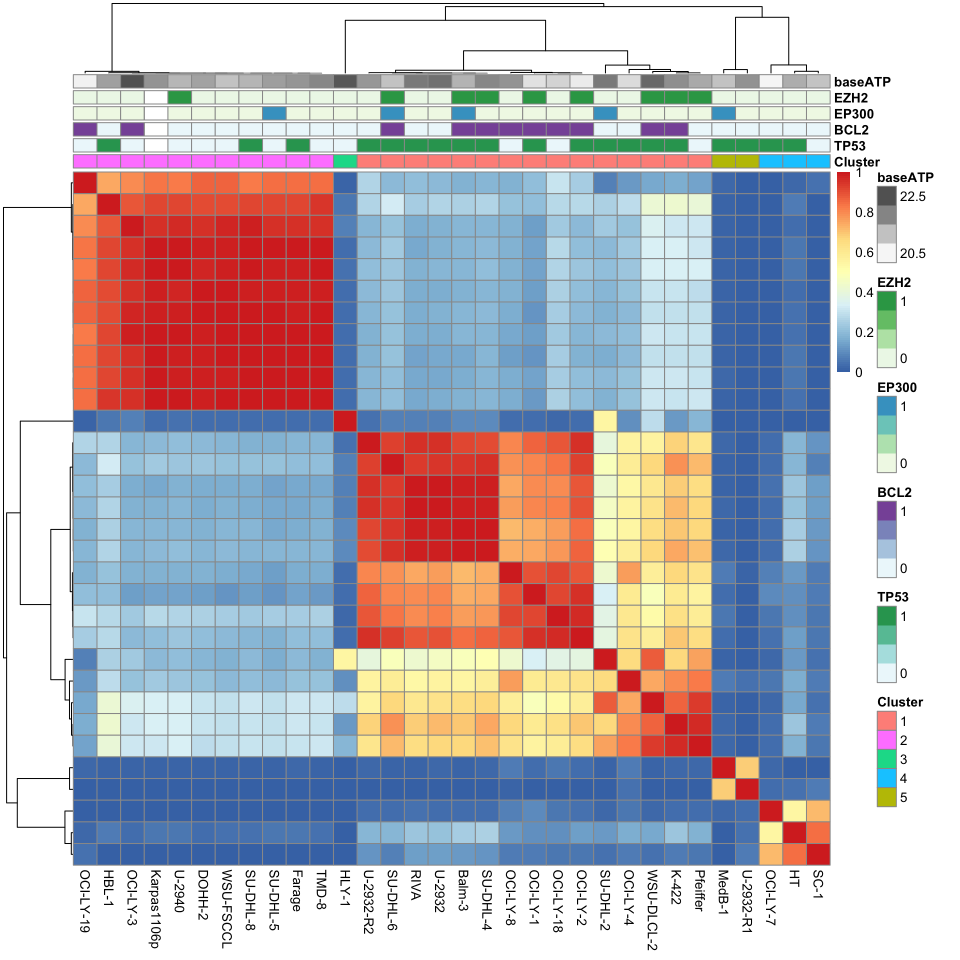
Visualize clusters in PCA
plotTab <- pcTab %>% mutate(cluster = conClust[Name])
ggplot(plotTab, aes(x=PC1, y=PC2, label = Name, col=factor(cluster))) +
  xlab(sprintf("PC1 (%1.1f%%)", 100*varExp[1])) + ylab(sprintf("PC2 (%1.1f%%)", 100*varExp[2])) +
  geom_point() +
  ggrepel::geom_text_repel()+
  theme_bw()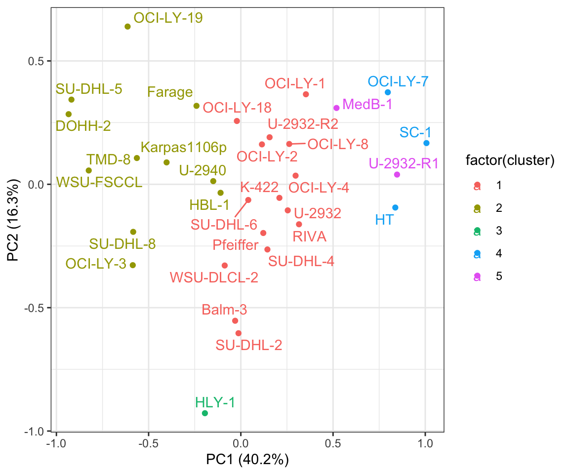
Visualize clusters in heatmap
colAnno <- colAnno[order(colAnno$Cluster),]


viabMat.order <- viabMat[,rownames(colAnno)]

#define color sequences
colorList <- c(colorRampPalette(c("navy", "white"))(20),
               colorRampPalette(c("white"))(5),
               colorRampPalette(c("white","firebrick3"))(20))

pheatmap(viabMat.order, scale = "row",
         clustering_method = "complete", annotation_col = colAnno,
         color = colorList,
         cluster_cols = FALSE,
         gaps_col = c(15,26,27,30,32))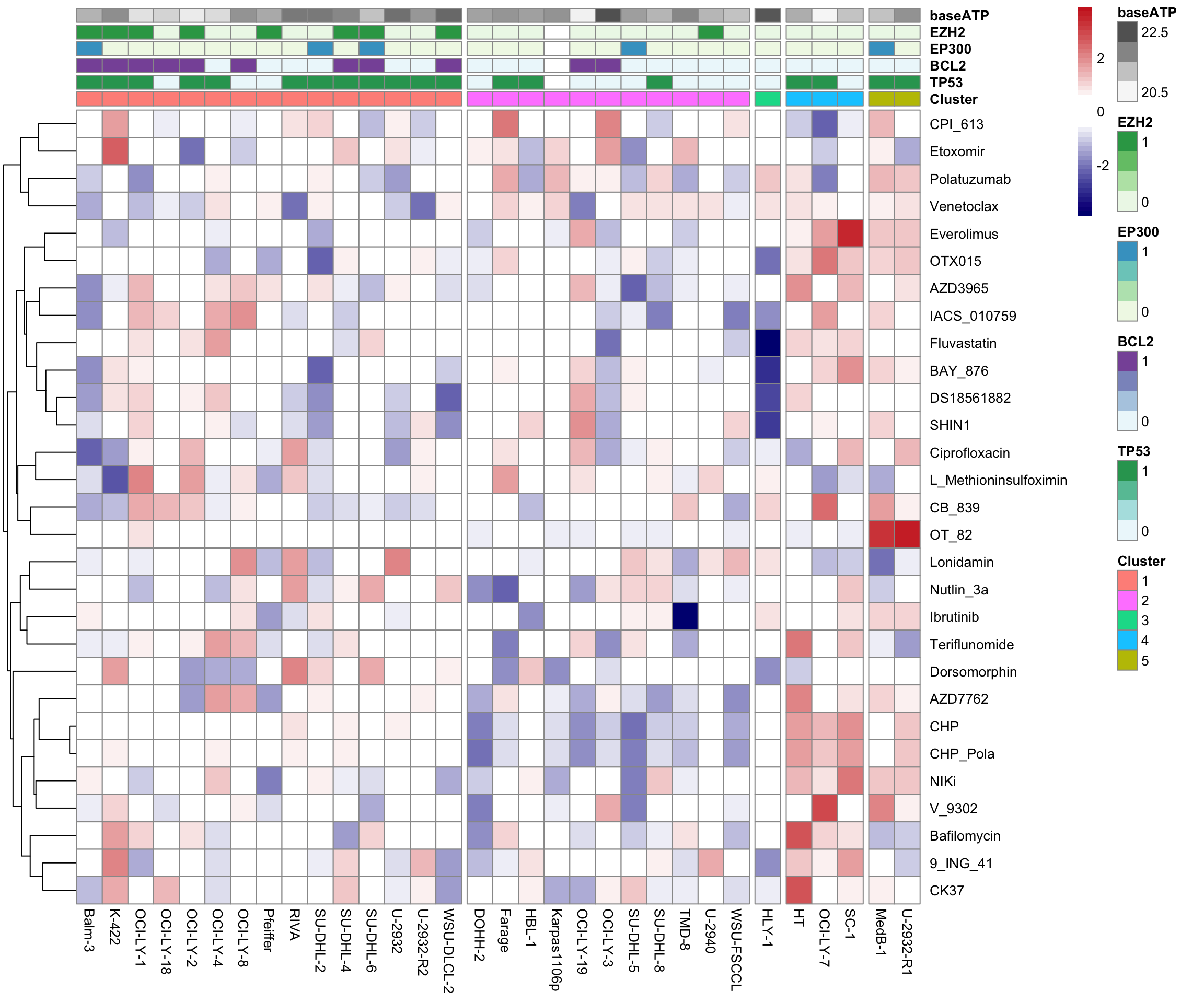
Identify signature drugs for the cluster
Only focus on cluster 1, 2 and 4, which have more then 3 samples
clusterTab <- tibble(Name = names(conClust), Cluster = conClust) %>%
  filter(Cluster %in% c(1,2,4)) %>%
  mutate(Cluster = paste0("C",Cluster))
ANOVA test
testTab <- viabTab %>% left_join(clusterTab, by = "Name") %>%
  filter(!is.na(Cluster)) %>% mutate(Cluster = factor(Cluster))

aovRes <- testTab %>% group_by(Drug) %>% nest() %>%
  mutate(m = map(data, ~lm(viab~Cluster,.))) %>%
  mutate(aov = map(m, car::Anova)) %>%
  mutate(res = map(aov, broom::tidy)) %>%
  unnest(res) %>%
  filter(term == "Cluster") %>%
  select(Drug, p.value) %>% arrange(p.value)
aovRes.sig <- filter(aovRes, p.value < 0.05)
Boxplot of significant associations
pList <- lapply(seq(nrow(aovRes.sig)), function(i) {
rec <- aovRes.sig[i,]
plotTab <- filter(testTab, Drug == rec$Drug) %>%
mutate(TP53 = factor(colAnno[Name,]$TP53)) %>%
filter(!is.na(TP53))
ggplot(plotTab, aes(x=Cluster, y=viab)) +
geom_boxplot(outlier.shape = NA) +
ggbeeswarm::geom_quasirandom(aes(col = Cluster, shape = TP53),size=3) +
theme_bw() +
ggtitle(sprintf("%s (p=%s)", rec$Drug, formatC(rec$p.value, digits = 2)))
})
cowplot::plot_grid(plotlist= pList, ncol=2)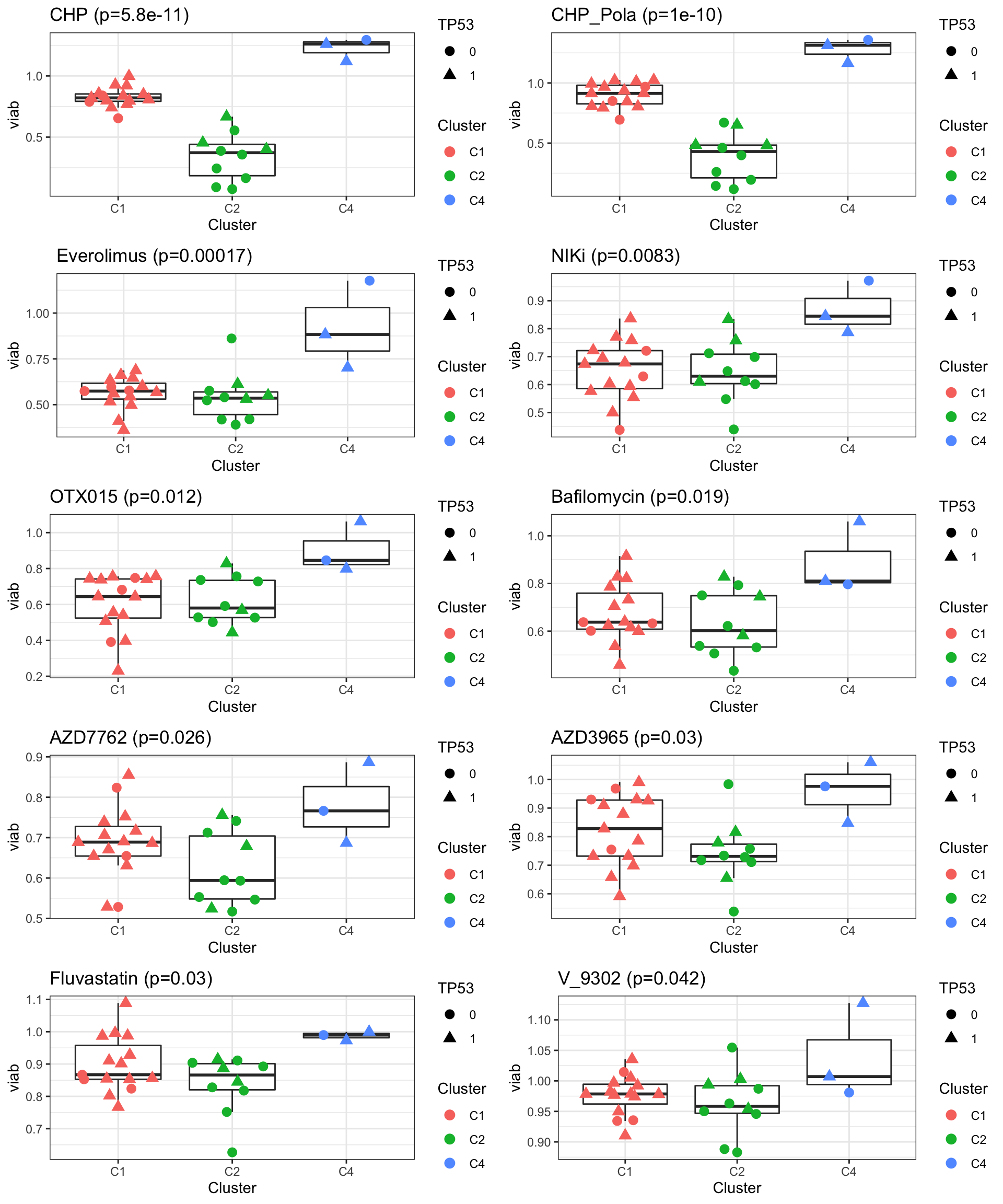 Basically C1 is the CHP resistant cluster and C2 is the CHP sensitive
cluster. The sensitively maybe related to TP53 mutations.
Basically C1 is the CHP resistant cluster and C2 is the CHP sensitive
cluster. The sensitively maybe related to TP53 mutations.
Association with proteomics/metabolomics
Proteomics
Data distribution
library(SummarizedExperiment)Loading required package: MatrixGenericsLoading required package: matrixStats
Attaching package: 'matrixStats'The following object is masked from 'package:dplyr':
count
Attaching package: 'MatrixGenerics'The following objects are masked from 'package:matrixStats':
colAlls, colAnyNAs, colAnys, colAvgsPerRowSet, colCollapse,
colCounts, colCummaxs, colCummins, colCumprods, colCumsums,
colDiffs, colIQRDiffs, colIQRs, colLogSumExps, colMadDiffs,
colMads, colMaxs, colMeans2, colMedians, colMins, colOrderStats,
colProds, colQuantiles, colRanges, colRanks, colSdDiffs, colSds,
colSums2, colTabulates, colVarDiffs, colVars, colWeightedMads,
colWeightedMeans, colWeightedMedians, colWeightedSds,
colWeightedVars, rowAlls, rowAnyNAs, rowAnys, rowAvgsPerColSet,
rowCollapse, rowCounts, rowCummaxs, rowCummins, rowCumprods,
rowCumsums, rowDiffs, rowIQRDiffs, rowIQRs, rowLogSumExps,
rowMadDiffs, rowMads, rowMaxs, rowMeans2, rowMedians, rowMins,
rowOrderStats, rowProds, rowQuantiles, rowRanges, rowRanks,
rowSdDiffs, rowSds, rowSums2, rowTabulates, rowVarDiffs, rowVars,
rowWeightedMads, rowWeightedMeans, rowWeightedMedians,
rowWeightedSds, rowWeightedVarsLoading required package: GenomicRangesLoading required package: stats4Loading required package: BiocGenerics
Attaching package: 'BiocGenerics'The following objects are masked from 'package:dplyr':
combine, intersect, setdiff, unionThe following objects are masked from 'package:stats':
IQR, mad, sd, var, xtabsThe following objects are masked from 'package:base':
anyDuplicated, append, as.data.frame, basename, cbind, colnames,
dirname, do.call, duplicated, eval, evalq, Filter, Find, get, grep,
grepl, intersect, is.unsorted, lapply, Map, mapply, match, mget,
order, paste, pmax, pmax.int, pmin, pmin.int, Position, rank,
rbind, Reduce, rownames, sapply, setdiff, sort, table, tapply,
union, unique, unsplit, which.max, which.minLoading required package: S4Vectors
Attaching package: 'S4Vectors'The following objects are masked from 'package:dplyr':
first, renameThe following object is masked from 'package:tidyr':
expandThe following objects are masked from 'package:base':
expand.grid, I, unnameLoading required package: IRanges
Attaching package: 'IRanges'The following objects are masked from 'package:dplyr':
collapse, desc, sliceThe following object is masked from 'package:purrr':
reduceLoading required package: GenomeInfoDbLoading required package: BiobaseWelcome to Bioconductor
Vignettes contain introductory material; view with
'browseVignettes()'. To cite Bioconductor, see
'citation("Biobase")', and for packages 'citation("pkgname")'.
Attaching package: 'Biobase'The following object is masked from 'package:MatrixGenerics':
rowMediansThe following objects are masked from 'package:matrixStats':
anyMissing, rowMediansprotData <- readRDS("../data/SC005_SummarizedExperiment_proteomics.RDS")
#select baseline samples
protData <- protData[,protData$condition %in% "U"]
protMat <- assay(protData)
boxplot(protMat)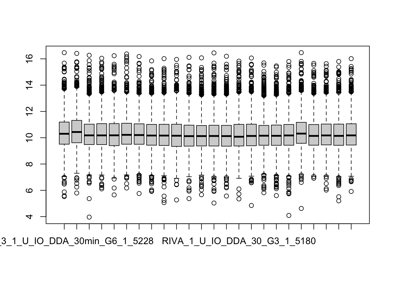
Median normalization (not performed)
#protMatNorm <- PhosR::medianScaling(protMat, scale = FALSE)
protMatNorm <- protMat
boxplot(protMatNorm)
protNorm <- protData
assay(protNorm) <- protMatNorm
Correlation between doxorubicine response and CHP response
patTab <- colData(protNorm) %>% as_tibble(rownames = "id") %>%
  mutate(viabCHP = viabMat["CHP",match(cell.line,colnames(viabMat))],
         cluster = clusterTab[match(cell.line, clusterTab$Name),]$Cluster,
         TP53 = factor(colAnno[match(cell.line, rownames(colAnno)),]$TP53)) %>%
  distinct(cell.line, .keep_all = TRUE)

ggplot(patTab, aes(x=Doxo.response, y=viabCHP, label = cell.line)) +
  geom_point(aes(col = cluster, shape = TP53)) +
  ggrepel::geom_text_repel(max.overlaps = Inf)
Warning: Removed 1 rows containing missing values (geom_point).Warning: Removed 1 rows containing missing values (geom_text_repel).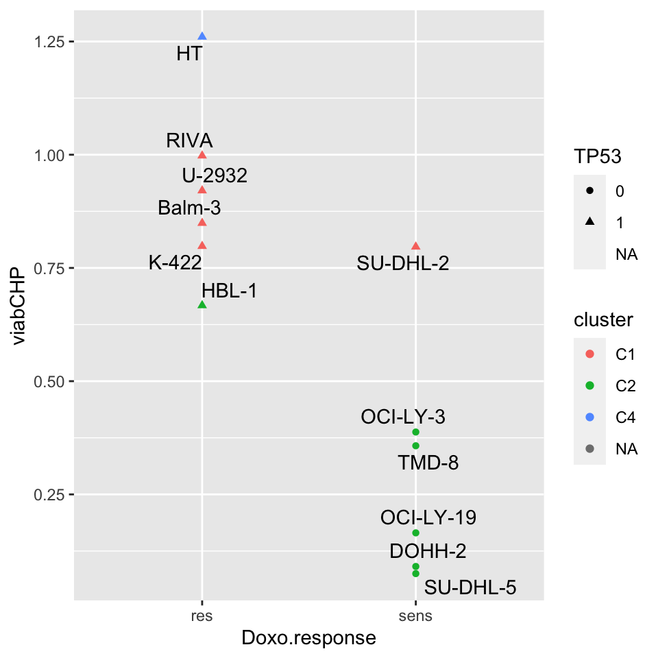
Average technical replicates for each cell line
protTab <- assay(protNorm) %>% as_tibble(rownames = "uniprotID") %>%
  pivot_longer(-uniprotID) %>%
  mutate(cellLine = colData(protNorm)[name,]$cell.line) %>%
  group_by(uniprotID, cellLine) %>%
  summarise(count = mean(value, na.rm=TRUE)) %>%
  mutate(symbol = rowData(protNorm)[uniprotID,]$Gene_name,
         cluster = clusterTab[match(cellLine, clusterTab$Name),]$Cluster,
         doxSense = colData(protNorm)[match(cellLine, protNorm$cell.line),]$Doxo.response) %>%
  filter(cellLine %in% clusterTab$Name,
         !symbol %in% c("",NA), !is.na(cluster)) %>%
  ungroup()
`summarise()` has grouped output by 'uniprotID'. You can override using the
`.groups` argument.protSub <- jyluMisc::tidyToSum(protTab, rowID = "uniprotID",colID = "cellLine",
values = "count", annoRow = "symbol",
annoCol = c("cluster", "doxSense"))
protSub$TP53 <- factor(colAnno[colnames(protSub),]$TP53)Identify proteins differentially expressed between C1 and C2
protSub <- protSub[,protSub$cluster %in% c("C1","C2")]
table(protSub$cluster)
C1 C2
 5  6
Differential protein expression using proDA
library(proDA)
protMat <- assay(protSub)
fit <- proDA(protMat, design = ~ cluster,
             col_data = colData(protSub))

resTab <- test_diff(fit, contrast = "clusterC2") %>%
  arrange(pval) %>%
  mutate(symbol = rowData(protSub[name,])$symbol)
hist(resTab$pval)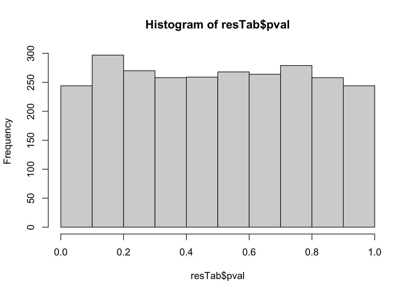 Not strong difference
Proteins with p-value < 0.05
resTab.sig <- filter(resTab, pval < 0.05)
resTab.sig %>% select(symbol, pval, adj_pval, diff) %>%
  mutate_if(is.numeric, formatC, digits=1) %>%
  DT::datatable()
Plot top 9 examples
pList <- lapply(seq(9), function(i) {
  rec <- resTab.sig[i,]
  plotTab <- tibble(expr = protMat[rec$name,],
                    cluster = protSub$cluster,
                    TP53 = protSub$TP53)
  ggplot(plotTab, aes(x=cluster, y=expr)) +
    geom_boxplot(outlier.shape = NA) +
    ggbeeswarm::geom_quasirandom(aes(color = cluster, shape = TP53), size=3) +
    ggtitle(rec$symbol) +
    theme_bw()
})

cowplot::plot_grid(plotlist = pList,ncol=3)
Warning: Removed 2 rows containing non-finite values (stat_boxplot).Warning: Removed 2 rows containing missing values (position_quasirandom).Warning: Removed 1 rows containing non-finite values (stat_boxplot).Warning: Removed 1 rows containing missing values (position_quasirandom).Warning: Removed 2 rows containing non-finite values (stat_boxplot).Warning: Removed 2 rows containing missing values (position_quasirandom).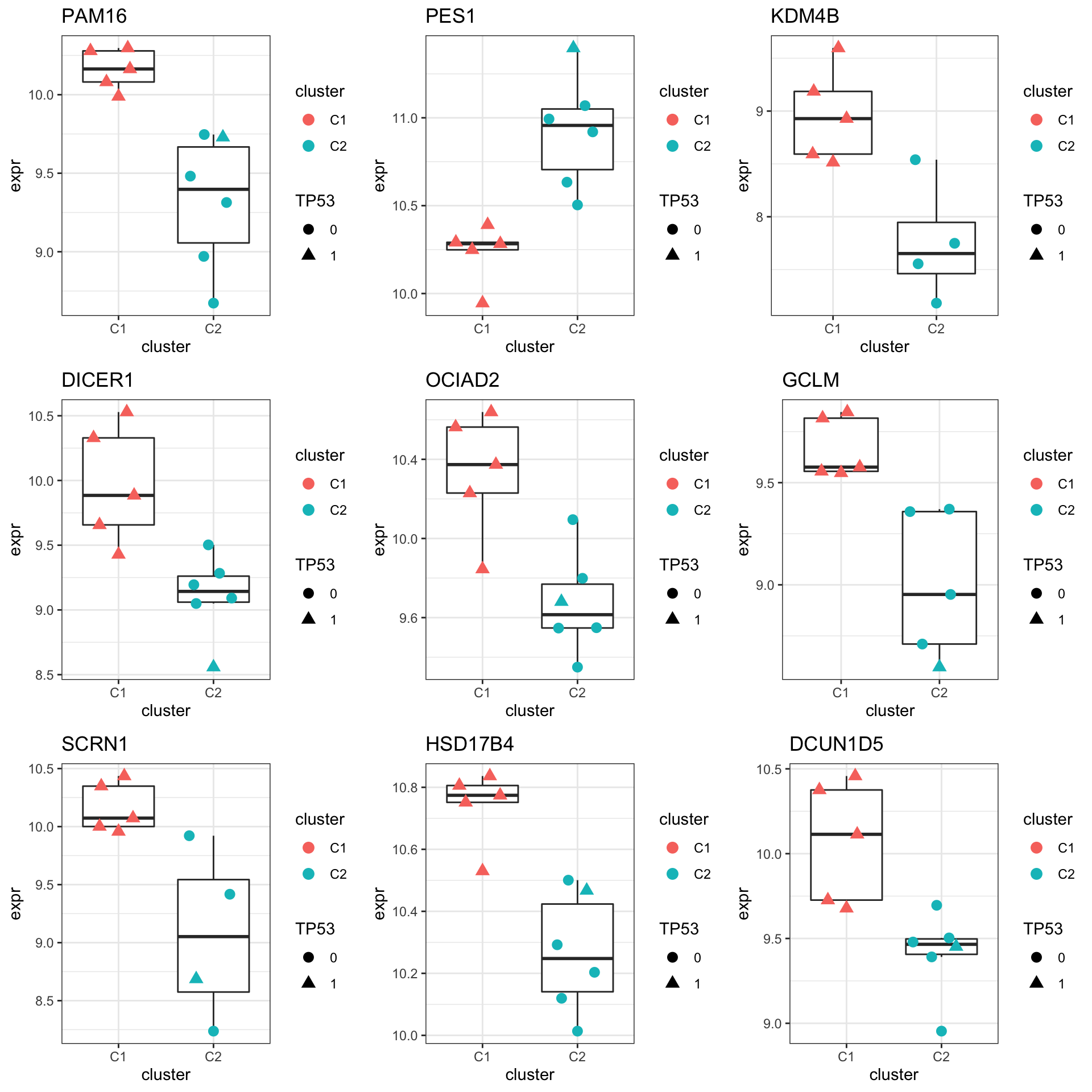
Enrichment analysis
gmts = list(H= "../data/gmts/h.all.v6.2.symbols.gmt",
            KEGG = "../data/gmts/c2.cp.kegg.v6.2.symbols.gmt",
            C6 = "../data/gmts/c6.all.v6.2.symbols.gmt")
inputTab <- resTab %>% filter(pval < 0.1) %>%
  distinct(symbol, .keep_all = TRUE) %>%
  select(symbol, t_statistic) %>% data.frame() %>% column_to_rownames("symbol")
enRes <- list()
enRes[["Hallmark"]] <- runGSEA(inputTab, gmts$H, "page")
Loading required package: pianoenRes[["KEGG"]] <- runGSEA(inputTab, gmts$KEGG,"page")
enRes[["Perturbation"]] <- runGSEA(inputTab, gmts$C6,"page")
p <- plotEnrichmentBar(enRes, pCut =0.01, ifFDR= FALSE)Coordinate system already present. Adding new coordinate system, which will replace the existing one.Coordinate system already present. Adding new coordinate system, which will replace the existing one.
Coordinate system already present. Adding new coordinate system, which will replace the existing one.cowplot::plot_grid(p)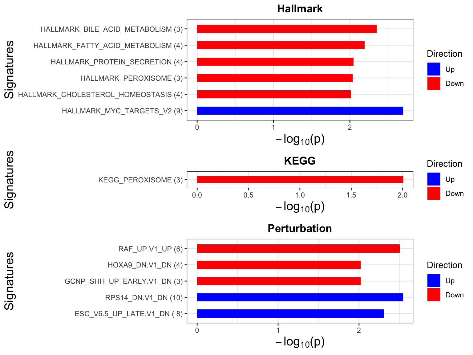
Focus on proteins from Fatty acid metabolism pathway
geneList <- piano::loadGSC(gmts$H)$gsc$HALLMARK_FATTY_ACID_METABOLISM
plotGene <- filter(filter(resTab, pval <= 0.1), symbol%in% geneList )
pList <- lapply(seq(nrow(plotGene)), function(i) {
rec <- plotGene[i,]
plotTab <- tibble(expr = protMat[rec$name,],
cluster = protSub$cluster,
TP53 = protSub$TP53)
ggplot(plotTab, aes(x=cluster, y=expr)) +
geom_boxplot(outlier.shape = NA) +
ggbeeswarm::geom_quasirandom(aes(color = cluster, shape = TP53), size=3) +
ggtitle(rec$symbol) +
theme_bw()
})
cowplot::plot_grid(plotlist = pList,ncol=3)Warning: Removed 3 rows containing non-finite values (stat_boxplot).Warning: Removed 3 rows containing missing values (position_quasirandom).Warning: Removed 1 rows containing non-finite values (stat_boxplot).Warning: Removed 1 rows containing missing values (position_quasirandom).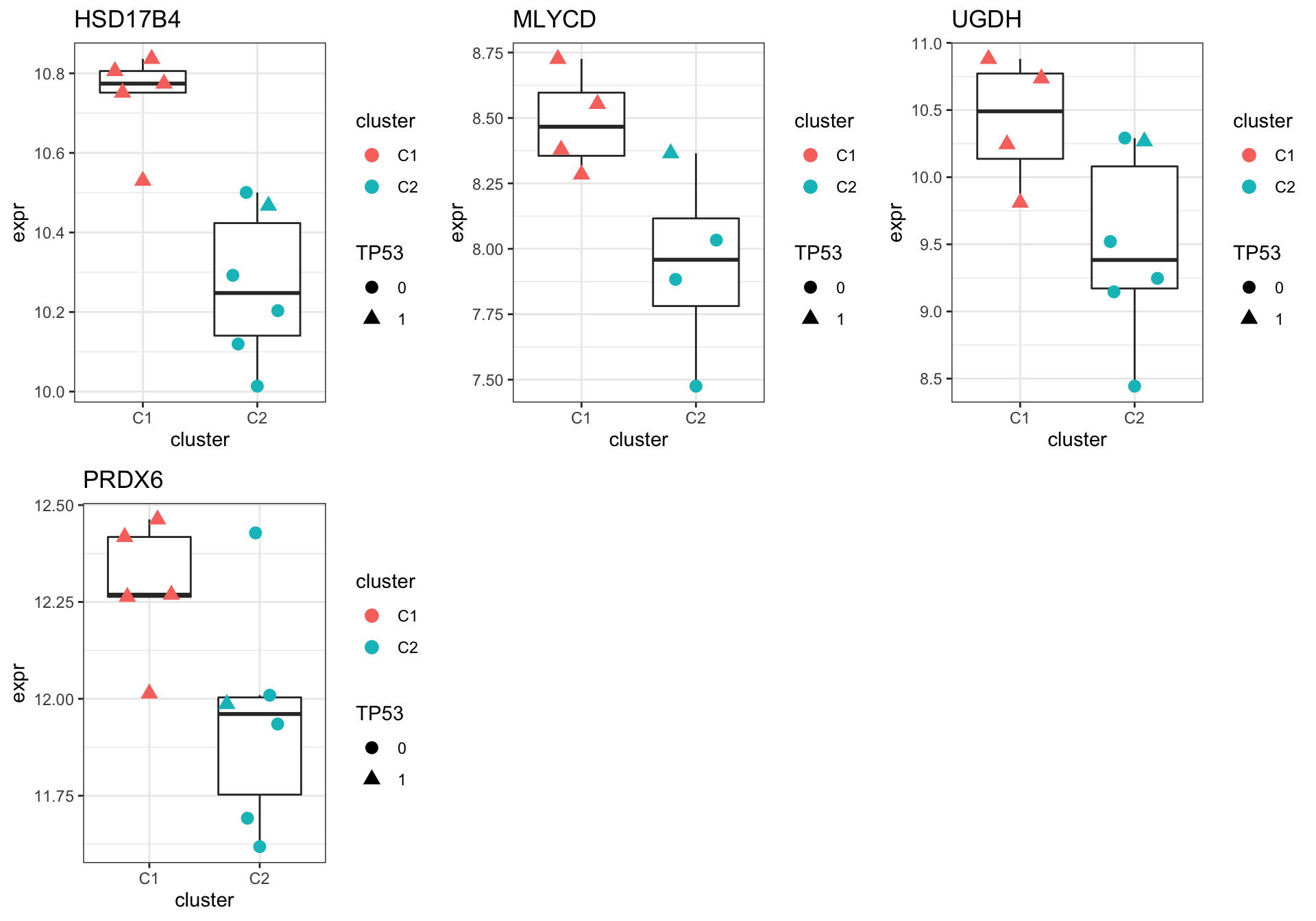
Proteomics (dataset from Tobias)
Data distribution
library(SummarizedExperiment)
load("../data/ProtWide.RData")
protMat <- ProtWideMedian normalization (not performed)
#protMatNorm <- PhosR::medianScaling(protMat, scale = FALSE)
protMatNorm <- protMat
boxplot(protMatNorm)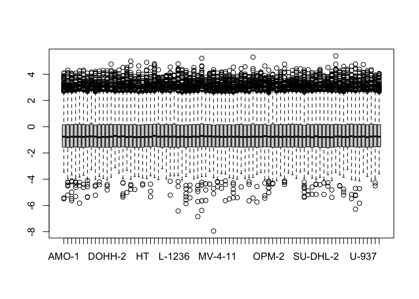
#protNorm <- protData
#assay(protNorm) <- protMatNormCreate assay experiment object
protTab <- protMatNorm %>% as_tibble(rownames = "uniprotID") %>%
pivot_longer(-uniprotID, names_to = "cellLine", values_to = "count") %>%
mutate(cluster = clusterTab[match(cellLine, clusterTab$Name),]$Cluster,
symbol = uniprotID) %>%
filter(cellLine %in% clusterTab$Name,
!symbol %in% c("",NA), !is.na(cluster))
protSub <- jyluMisc::tidyToSum(protTab, rowID = "uniprotID",colID = "cellLine",
values = "count", annoRow = "symbol", annoCol = "cluster")
protSub$TP53 <- factor(colAnno[colnames(protSub),]$TP53)Identify proteins differentially expressed between C1 and C2
protSub <- protSub[,protSub$cluster %in% c("C1","C2")]
table(protSub$cluster)
C1 C2
15 10 Differential protein expression using proDA
library(proDA)
protMat <- assay(protSub)
fit <- proDA(protMat, design = ~ cluster,
col_data = colData(protSub))
resTab <- test_diff(fit, contrast = "clusterC2") %>%
arrange(pval) %>%
mutate(symbol = rowData(protSub[name,])$symbol)hist(resTab$pval)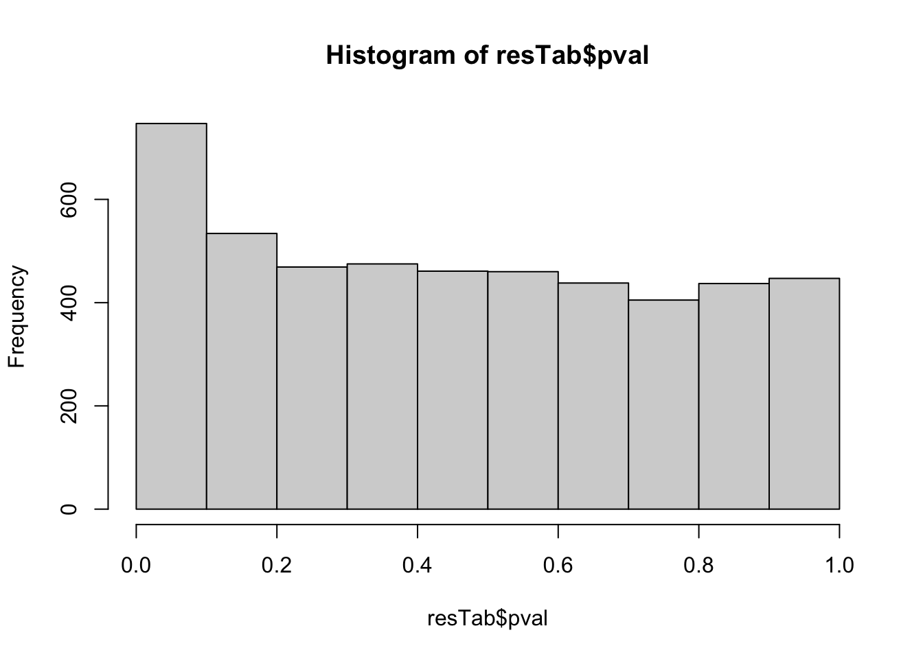 Stronger associations can be observed
Proteins with p-value < 0.05
resTab.sig <- filter(resTab, pval < 0.05)
resTab.sig %>% select(symbol, pval, adj_pval, diff) %>%
mutate_if(is.numeric, formatC, digits=1) %>%
DT::datatable()Plot top 9 examples
pList <- lapply(seq(9), function(i) {
rec <- resTab.sig[i,]
plotTab <- tibble(expr = protMat[rec$name,],
cluster = protSub$cluster,
TP53 = protSub$TP53)
ggplot(plotTab, aes(x=cluster, y=expr)) +
geom_boxplot(outlier.shape = NA) +
ggbeeswarm::geom_quasirandom(aes(color = cluster, shape = TP53), size=3) +
ggtitle(rec$symbol) +
theme_bw()
})
cowplot::plot_grid(plotlist = pList,ncol=3)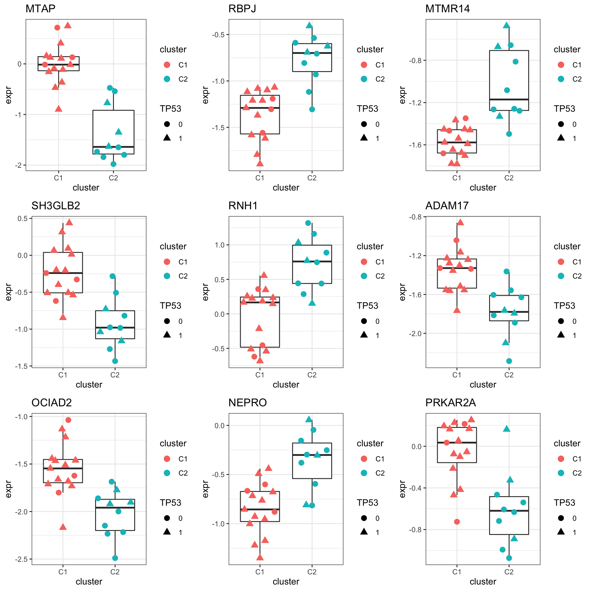
Enrichment analysis
gmts = list(H= "../data/gmts/h.all.v6.2.symbols.gmt",
KEGG = "../data/gmts/c2.cp.kegg.v6.2.symbols.gmt",
C6 = "../data/gmts/c6.all.v6.2.symbols.gmt")
inputTab <- resTab %>% filter(pval < 0.1) %>%
distinct(symbol, .keep_all = TRUE) %>%
select(symbol, t_statistic) %>% data.frame() %>% column_to_rownames("symbol")
enRes <- list()
enRes[["Hallmark"]] <- runGSEA(inputTab, gmts$H, "page")
enRes[["KEGG"]] <- runGSEA(inputTab, gmts$KEGG,"page")
enRes[["Perturbation"]] <- runGSEA(inputTab, gmts$C6,"page")
p <- plotEnrichmentBar(enRes, pCut =0.05, ifFDR= FALSE)Coordinate system already present. Adding new coordinate system, which will replace the existing one.
Coordinate system already present. Adding new coordinate system, which will replace the existing one.
Coordinate system already present. Adding new coordinate system, which will replace the existing one.
cowplot::plot_grid(p)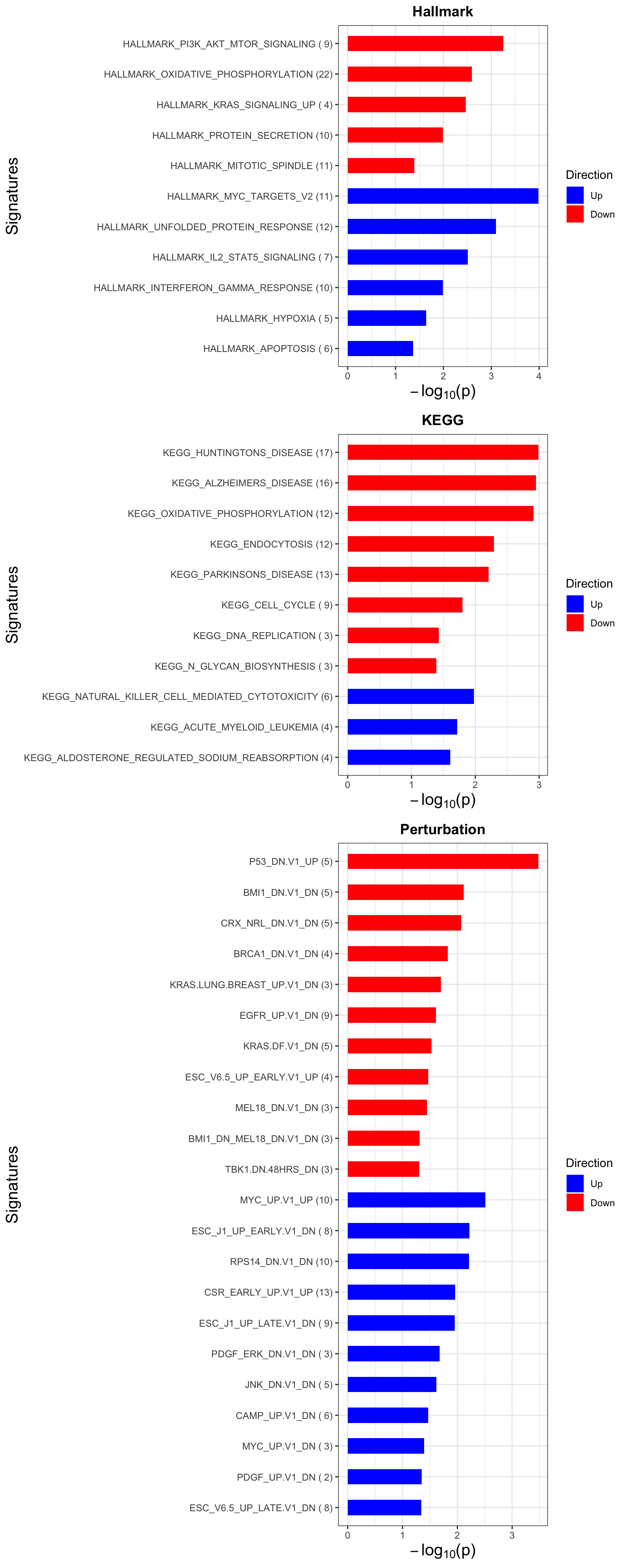
Focus on proteins from Fatty acid metabolism pathway
geneList <- piano::loadGSC(gmts$H)$gsc$HALLMARK_FATTY_ACID_METABOLISM
plotGene <- filter(filter(resTab, pval <= 0.05), symbol%in% geneList )
pList <- lapply(seq(nrow(plotGene)), function(i) {
  rec <- plotGene[i,]
  plotTab <- tibble(expr = protMat[rec$name,],
                    cluster = protSub$cluster,
                    TP53 = protSub$TP53)
  ggplot(plotTab, aes(x=cluster, y=expr)) +
    geom_boxplot(outlier.shape = NA) +
    ggbeeswarm::geom_quasirandom(aes(color = cluster, shape = TP53), size=3) +
    ggtitle(rec$symbol) +
    theme_bw()
})

cowplot::plot_grid(plotlist = pList,ncol=3)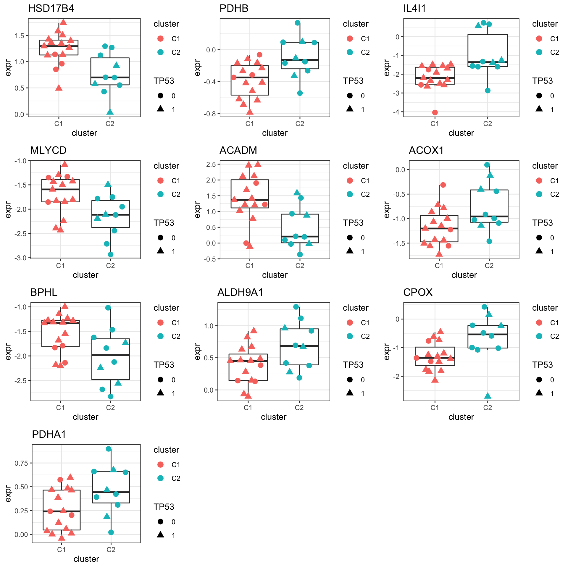
Metabolimics
Data distribution
metaData <- readRDS("../data/SC005_SummarizedExperiment_metabolomics.RDS")
metaMat <- assay(metaData)
boxplot(metaMat)
Median normalization (not performed)
#metaMatNorm <- PhosR::medianScaling(metaMat, scale = FALSE)
metaMatNorm <- metaMat
boxplot(metaMatNorm)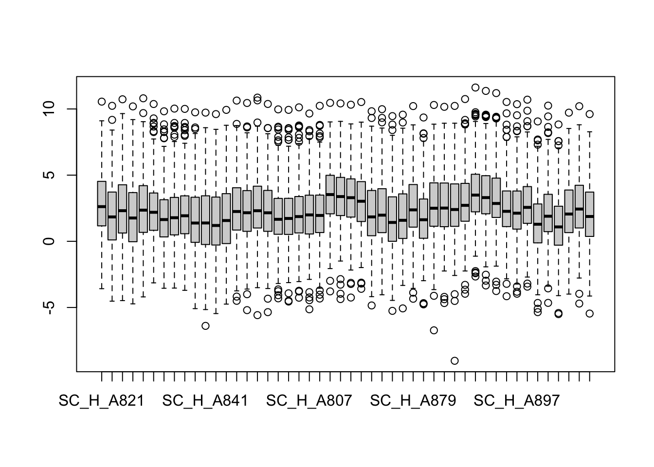
metaNorm <- metaData
assay(metaNorm) <- metaMatNorm
Average technical replicates for each cell line
metaTab <- assay(metaNorm) %>% as_tibble(rownames = "id") %>%
  pivot_longer(-id) %>%
  mutate(cellLine = colData(metaNorm)[name,]$cell.line) %>%
  group_by(id, cellLine) %>%
  summarise(count = mean(value, na.rm=TRUE)) %>%
  mutate(symbol = rowData(metaNorm)[id,]$metabolite,
         class = rowData(metaNorm)[id,]$class,
         cluster = clusterTab[match(cellLine, clusterTab$Name),]$Cluster) %>%
  filter(cellLine %in% clusterTab$Name,
         !symbol %in% c("",NA), !is.na(cluster))
`summarise()` has grouped output by 'id'. You can override using the `.groups`
argument.metaSub <- jyluMisc::tidyToSum(metaTab, rowID = "id",colID = "cellLine",
values = "count", annoRow = c("symbol","class"), annoCol = "cluster")
metaSub$TP53 <- factor(colAnno[colnames(metaSub),]$TP53)Identify proteins differentially expressed between C1 and C2
metaSub <- metaSub[,metaSub$cluster %in% c("C1","C2")]
table(metaSub$cluster)
C1 C2
 5  6
Differential metabolites abundance
library(limma)
metaMat <- assay(metaSub)
designMat <- model.matrix(~metaSub$cluster)
fit <- lmFit(metaMat, designMat)
fit2 <- eBayes(fit)

resTab <- topTable(fit2, number= Inf) %>%
  dplyr::rename(pval = P.Value, adj_pval = adj.P.Val) %>%
  arrange(pval) %>%
  as_tibble(rownames = "name") %>%
  mutate(symbol = rowData(metaSub[name,])$symbol)
hist(resTab$pval) Not strong difference
Proteins with p-value < 0.05
resTab.sig <- filter(resTab, pval < 0.05)
resTab.sig %>% select(symbol, pval, adj_pval, logFC, t) %>%
  mutate_if(is.numeric, formatC, digits=1) %>%
  DT::datatable()
Plot top 9 examples
pList <- lapply(seq(9), function(i) {
  rec <- resTab.sig[i,]
  plotTab <- tibble(expr = metaMat[rec$name,],
                    cluster = metaSub$cluster,
                    TP53 = metaSub$TP53)
  ggplot(plotTab, aes(x=cluster, y=expr)) +
    geom_boxplot(outlier.shape = NA) +
    ggbeeswarm::geom_quasirandom(aes(color = cluster, shape = TP53), size=3) +
    ggtitle(rec$symbol) +
    theme_bw()
})

cowplot::plot_grid(plotlist = pList,ncol=3)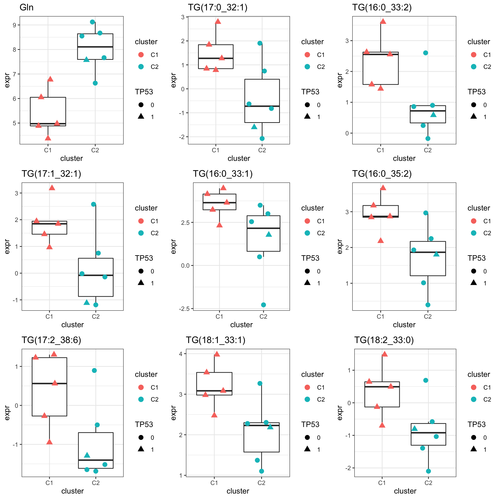
sessionInfo()R version 4.2.0 (2022-04-22)
Platform: x86_64-apple-darwin17.0 (64-bit)
Running under: macOS Big Sur/Monterey 10.16
Matrix products: default
BLAS: /Library/Frameworks/R.framework/Versions/4.2/Resources/lib/libRblas.0.dylib
LAPACK: /Library/Frameworks/R.framework/Versions/4.2/Resources/lib/libRlapack.dylib
locale:
[1] en_US.UTF-8/en_US.UTF-8/en_US.UTF-8/C/en_US.UTF-8/en_US.UTF-8
attached base packages:
[1] stats4 stats graphics grDevices utils datasets methods
[8] base
other attached packages:
[1] limma_3.52.2 piano_2.12.0
[3] proDA_1.10.0 SummarizedExperiment_1.26.1
[5] Biobase_2.56.0 GenomicRanges_1.48.0
[7] GenomeInfoDb_1.32.2 IRanges_2.30.0
[9] S4Vectors_0.34.0 BiocGenerics_0.42.0
[11] MatrixGenerics_1.8.0 matrixStats_0.62.0
[13] ConsensusClusterPlus_1.60.0 pheatmap_1.0.12
[15] forcats_0.5.1 stringr_1.4.0
[17] dplyr_1.0.9 purrr_0.3.4
[19] readr_2.1.2 tidyr_1.2.0
[21] tibble_3.1.7 ggplot2_3.3.6
[23] tidyverse_1.3.1 jyluMisc_0.1.5
loaded via a namespace (and not attached):
[1] readxl_1.4.0 backports_1.4.1 fastmatch_1.1-3
[4] drc_3.0-1 workflowr_1.7.0 igraph_1.3.2
[7] shinydashboard_0.7.2 splines_4.2.0 crosstalk_1.2.0
[10] BiocParallel_1.30.3 TH.data_1.1-1 digest_0.6.29
[13] htmltools_0.5.2 fansi_1.0.3 magrittr_2.0.3
[16] cluster_2.1.3 tzdb_0.3.0 modelr_0.1.8
[19] sandwich_3.0-2 colorspace_2.0-3 ggrepel_0.9.1
[22] rvest_1.0.2 haven_2.5.0 xfun_0.31
[25] crayon_1.5.1 RCurl_1.98-1.7 jsonlite_1.8.0
[28] survival_3.3-1 zoo_1.8-10 glue_1.6.2
[31] survminer_0.4.9 gtable_0.3.0 zlibbioc_1.42.0
[34] XVector_0.36.0 DelayedArray_0.22.0 car_3.1-0
[37] abind_1.4-5 scales_1.2.0 mvtnorm_1.1-3
[40] DBI_1.1.3 relations_0.6-12 rstatix_0.7.0
[43] Rcpp_1.0.8.3 plotrix_3.8-2 xtable_1.8-4
[46] km.ci_0.5-6 DT_0.23 htmlwidgets_1.5.4
[49] httr_1.4.3 fgsea_1.22.0 RColorBrewer_1.1-3
[52] gplots_3.1.3 ellipsis_0.3.2 farver_2.1.0
[55] pkgconfig_2.0.3 sass_0.4.1 dbplyr_2.2.0
[58] utf8_1.2.2 tidyselect_1.1.2 labeling_0.4.2
[61] rlang_1.0.2 later_1.3.0 munsell_0.5.0
[64] cellranger_1.1.0 tools_4.2.0 visNetwork_2.1.0
[67] cli_3.3.0 generics_0.1.2 broom_0.8.0
[70] evaluate_0.15 fastmap_1.1.0 yaml_2.3.5
[73] knitr_1.39 fs_1.5.2 survMisc_0.5.6
[76] caTools_1.18.2 mime_0.12 slam_0.1-50
[79] xml2_1.3.3 compiler_4.2.0 rstudioapi_0.13
[82] beeswarm_0.4.0 ggsignif_0.6.3 marray_1.74.0
[85] reprex_2.0.1 bslib_0.3.1 stringi_1.7.6
[88] highr_0.9 lattice_0.20-45 Matrix_1.4-1
[91] shinyjs_2.1.0 KMsurv_0.1-5 vctrs_0.4.1
[94] pillar_1.7.0 lifecycle_1.0.1 jquerylib_0.1.4
[97] data.table_1.14.2 cowplot_1.1.1 bitops_1.0-7
[100] httpuv_1.6.5 extraDistr_1.9.1 R6_2.5.1
[103] promises_1.2.0.1 KernSmooth_2.23-20 gridExtra_2.3
[106] vipor_0.4.5 codetools_0.2-18 MASS_7.3-57
[109] gtools_3.9.2.2 exactRankTests_0.8-35 assertthat_0.2.1
[112] rprojroot_2.0.3 withr_2.5.0 multcomp_1.4-19
[115] GenomeInfoDbData_1.2.8 parallel_4.2.0 hms_1.1.1
[118] grid_4.2.0 rmarkdown_2.14 carData_3.0-5
[121] git2r_0.30.1 maxstat_0.7-25 ggpubr_0.4.0
[124] sets_1.0-21 shiny_1.7.1 lubridate_1.8.0
[127] ggbeeswarm_0.6.0