Exploretory data analysis of the whole dataset
Junyan Lu
Last updated: 2022-11-10
Checks: 5 1
Knit directory: irAE_LungCancer/analysis/
This reproducible R Markdown analysis was created with workflowr (version 1.7.0). The Checks tab describes the reproducibility checks that were applied when the results were created. The Past versions tab lists the development history.
Great job! The global environment was empty. Objects defined in the global environment can affect the analysis in your R Markdown file in unknown ways. For reproduciblity it’s best to always run the code in an empty environment.
The command set.seed(20221110) was run prior to running
the code in the R Markdown file. Setting a seed ensures that any results
that rely on randomness, e.g. subsampling or permutations, are
reproducible.
Great job! Recording the operating system, R version, and package versions is critical for reproducibility.
Nice! There were no cached chunks for this analysis, so you can be confident that you successfully produced the results during this run.
Great job! Using relative paths to the files within your workflowr project makes it easier to run your code on other machines.
Tracking code development and connecting the code version to the
results is critical for reproducibility. To start using Git, open the
Terminal and type git init in your project directory.
This project is not being versioned with Git. To obtain the full
reproducibility benefits of using workflowr, please see
?wflow_start.
The purpose of this analysis is to understand the overall structure of the data
Load data packages
library(MultiAssayExperiment)
library(pheatmap)
library(vsn)
library(tidyverse)
knitr::opts_chunk$set(warning = FALSE, message = FALSE)

load("../output/processedData.RData")
patAnno <- colData(mae) %>%
    as_tibble(rownames = "sampleID")
CBA data
Data distribution
Per sample
cbaTab <- filter(fullTab, assay == "CBA")

ggplot(cbaTab, aes(x=sampleID, y=value)) +
    geom_point() +
    theme(axis.text.x = element_text(angle = 90, hjust = 1, vjust = 0.5))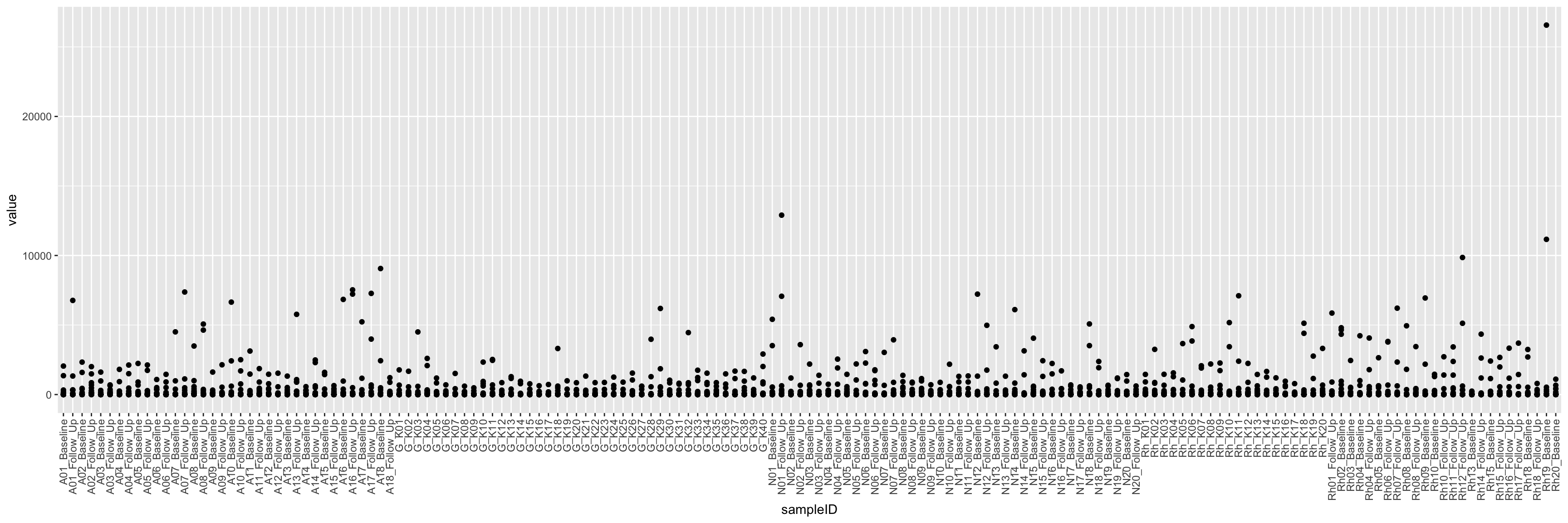
Per feature
ggplot(cbaTab, aes(x=name, y=value)) +
    geom_point() +
    theme(axis.text.x = element_text(angle = 90, hjust = 1, vjust = 0.5))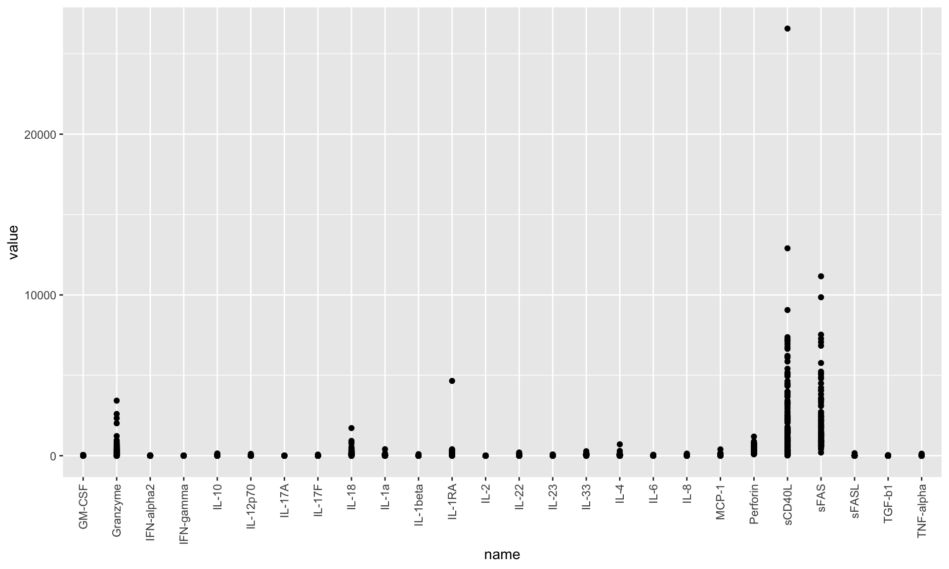
glog2 transformation
(generalized log2 transformation to deal with 0s)
Per feature
cbaTab <- mutate(cbaTab, logVal = jyluMisc::glog2(value))
ggplot(cbaTab, aes(x=name, y=logVal)) +
    geom_point() +
    theme(axis.text.x = element_text(angle = 90, hjust = 1, vjust = 0.5))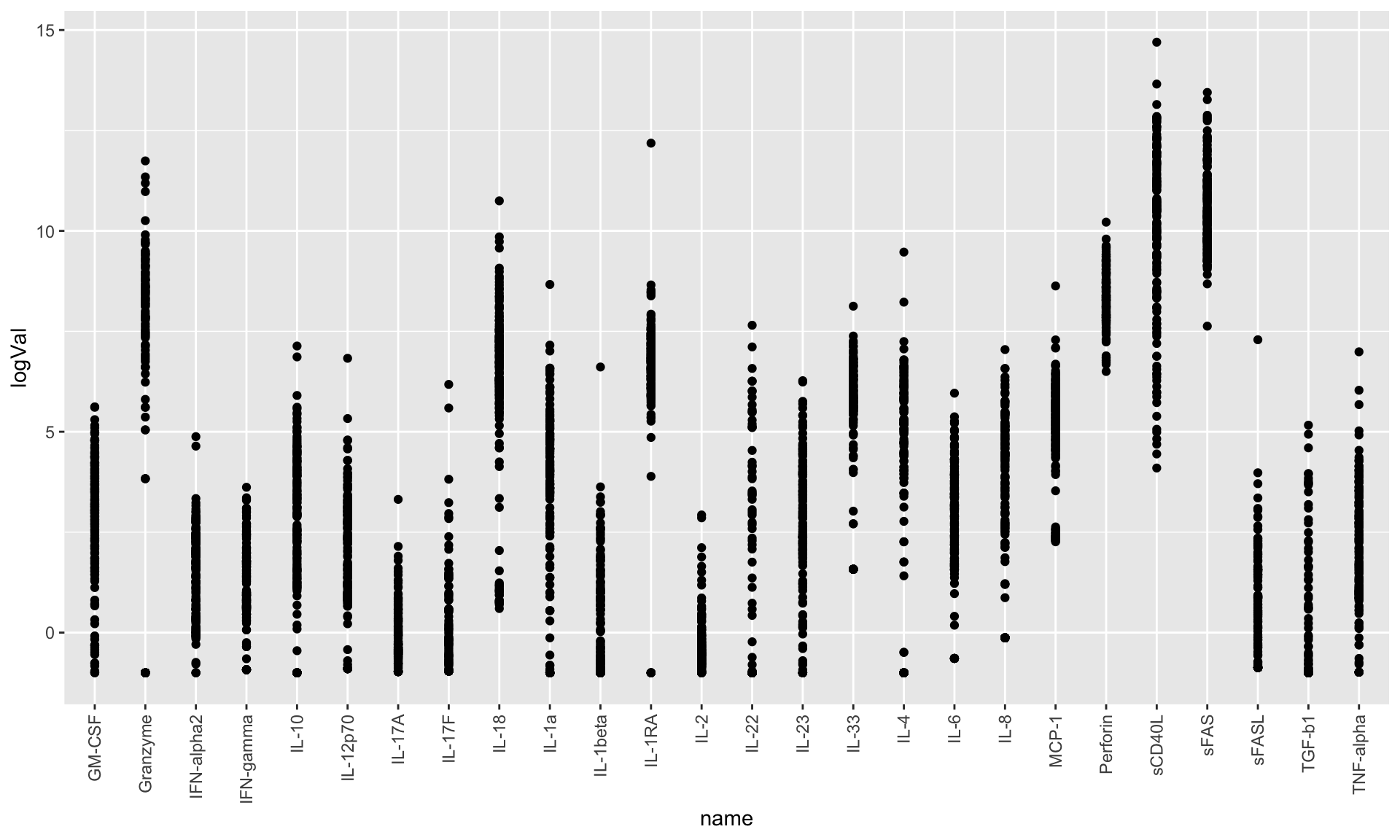
Per sample
ggplot(cbaTab, aes(x=sampleID, y=logVal)) +
    geom_boxplot(outlier.shape = NA) +
    geom_point(size=0.5) +
    theme(axis.text.x = element_text(angle = 90, hjust = 1, vjust = 0.5))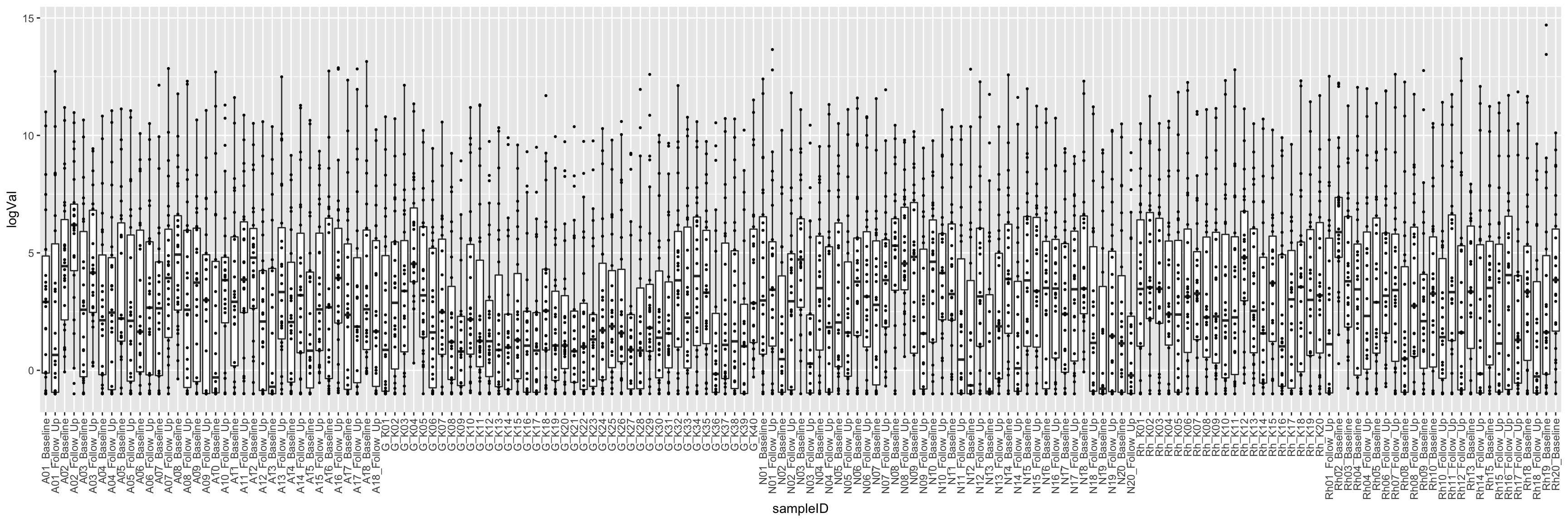
PCA analysis
Use log2 transformed data
Variance explained
dataMat <- jyluMisc::glog2(t(mae[["cba"]]))
pcRes <- prcomp(dataMat, center = TRUE, scale. = TRUE)
plotTab <- pcRes$x %>% as_tibble(rownames = "sampleID") %>%
    left_join(patAnno, by = "sampleID")

varExp <- pcRes$sdev^2/sum(pcRes$sdev^2)
varTab <- tibble(pc = colnames(pcRes$x), var = varExp*100) %>%
    mutate(pc = factor(pc, levels = pc))
ggplot(varTab, aes(x=pc, y=var)) +
    geom_bar(stat= "identity")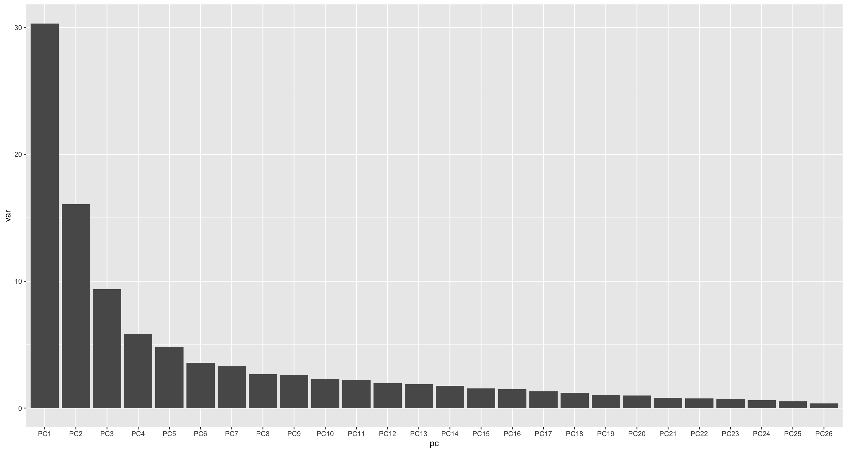
PC1 versus PC2
ggplot(plotTab, aes(x=PC1, y=PC2)) +
    geom_point(aes(color = Group, shape = condition), size=3) +
    geom_line(aes(group=patID), color = "grey50", linetype = "dotted")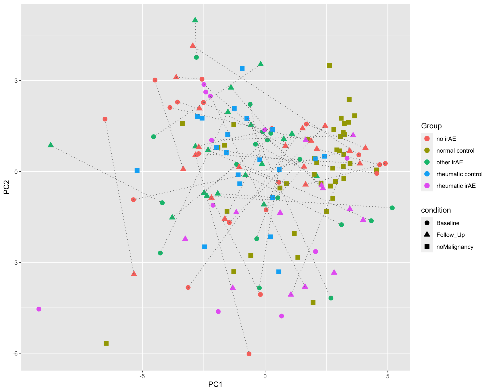
PC3 versus PC4
ggplot(plotTab, aes(x=PC3, y=PC4)) +
    geom_point(aes(color = Group, shape = condition), size=3) +
    geom_line(aes(group=patID), color = "grey50", linetype = "dotted")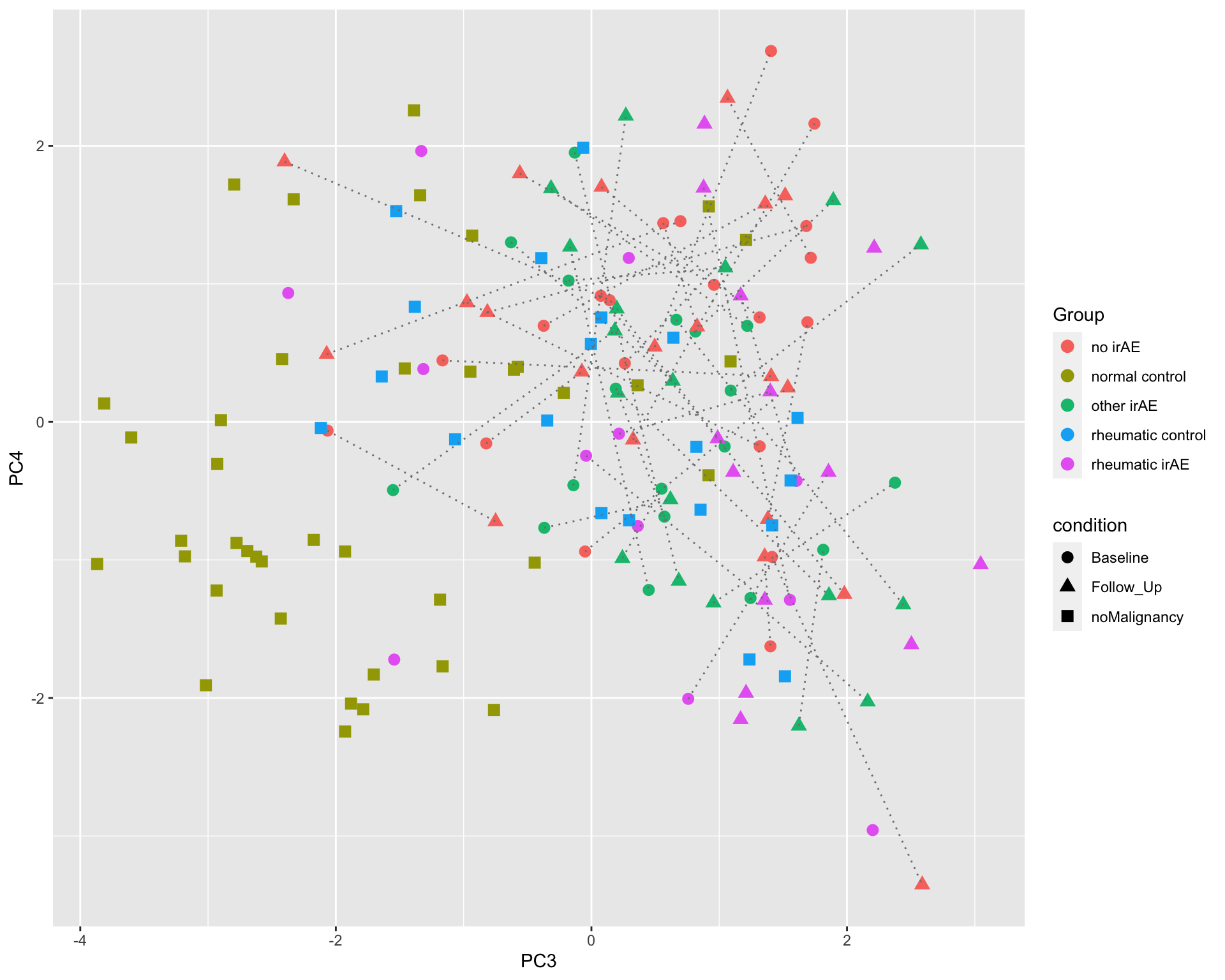
Correlated between PCs and metadata
pcTab <- pcRes$x[,1:20] %>% as_tibble(rownames = "smpID")
metaTab <- colData(mae) %>% as_tibble(rownames = "smpID")
corRes <- jyluMisc::testAssociation(pcTab, metaTab, "smpID")
head(corRes, n=20)
var1 var2 p
1 PC3 dateOfAcquisition_CBA 4.438659e-22
2 PC3 Group 2.604577e-17
3 PC3 dateOfAcquisition_NMR 3.521165e-15
4 PC3 condition 1.035028e-13
5 PC3 Tumor 4.259001e-12
6 PC1 dateOfAcquisition_CBA 9.697376e-08
7 PC4 dateOfAcquisition_CBA 1.223884e-06
8 PC3 patID 3.261982e-05
9 PC17 Malignoma.Duration.at.Baseline 4.675033e-05
10 PC4 Gender 7.727792e-05
11 PC8 patID 1.013612e-04
12 PC7 Height 1.046023e-04
13 PC9 Age.at.irAE.diagnosis 2.391630e-04
14 PC1 Group 2.617779e-04
15 PC5 Surgery 3.583696e-04
16 PC13 condition 5.297203e-04
17 PC16 Rheumatoid.Factor 7.379344e-04
18 PC7 Gender 8.119075e-04
19 PC4 Height 9.705809e-04
20 PC20 Preexisting.RMD 1.373438e-03ggplot(plotTab, aes(x=PC1, y=PC3)) +
geom_point(aes(color = factor(dateOfAcquisition_CBA), shape = Group), size=3) +
geom_line(aes(group=patID), color = "grey50", linetype = "dotted")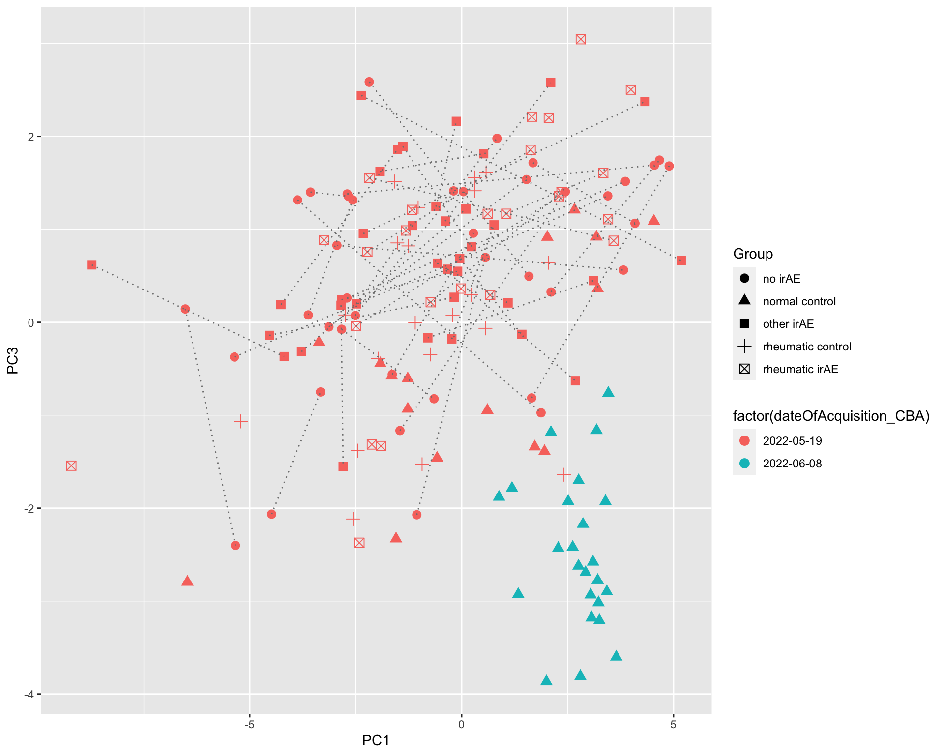 There’s potentially a confounding between date of acquisition
Clustering
Without scaling
annoCol <- colData(mae)[,c("condition","Group","Gender", "dateOfAcquisition_CBA")] %>% data.frame()
annoCol$dateOfAcquisition_CBA <- as.character(annoCol$dateOfAcquisition_CBA)
pheatmap(dataMat, annotation_row = annoCol, clustering_method = "ward.D2")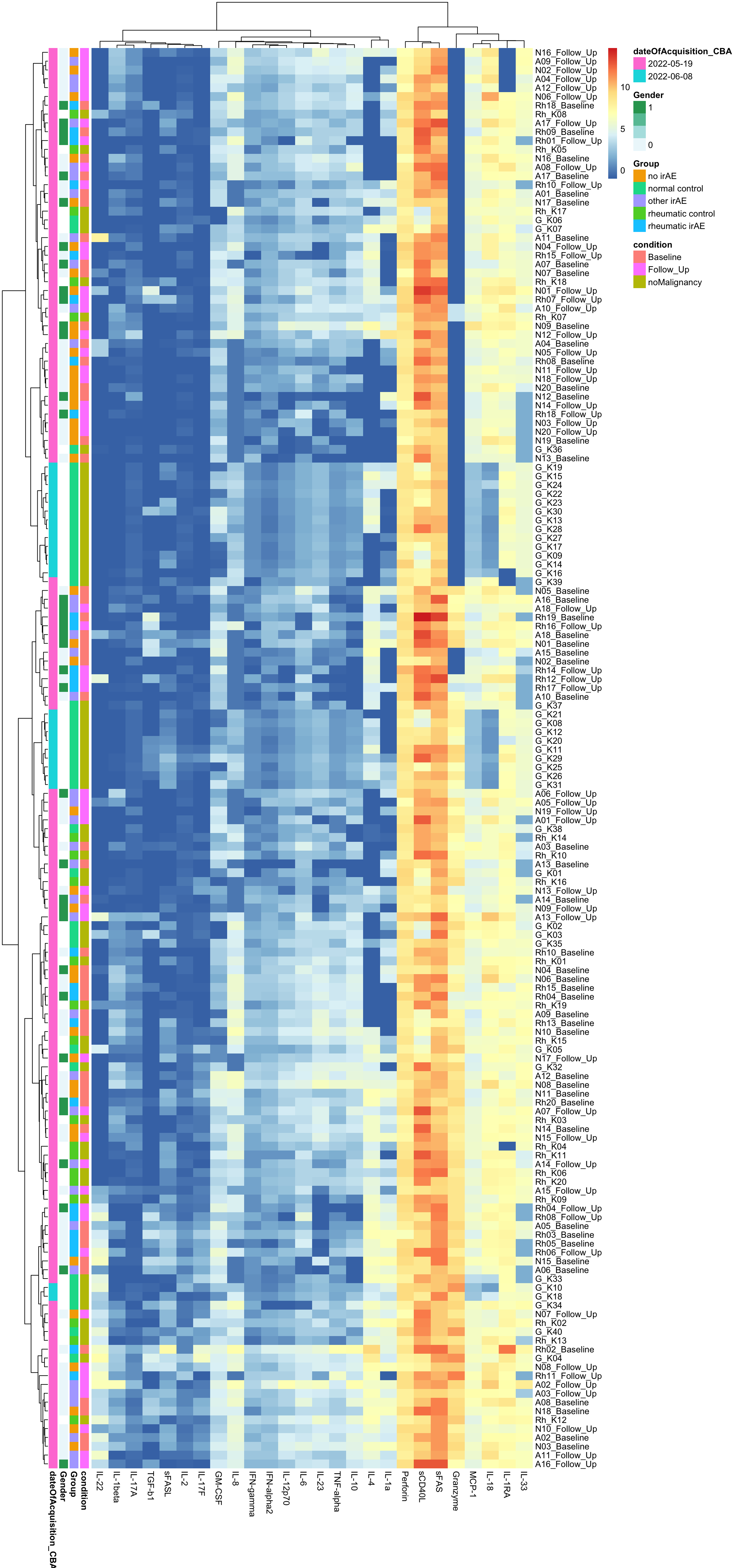
Column Scaled
pheatmap(dataMat, annotation_row = annoCol, scale="column", clustering_method = "ward.D2")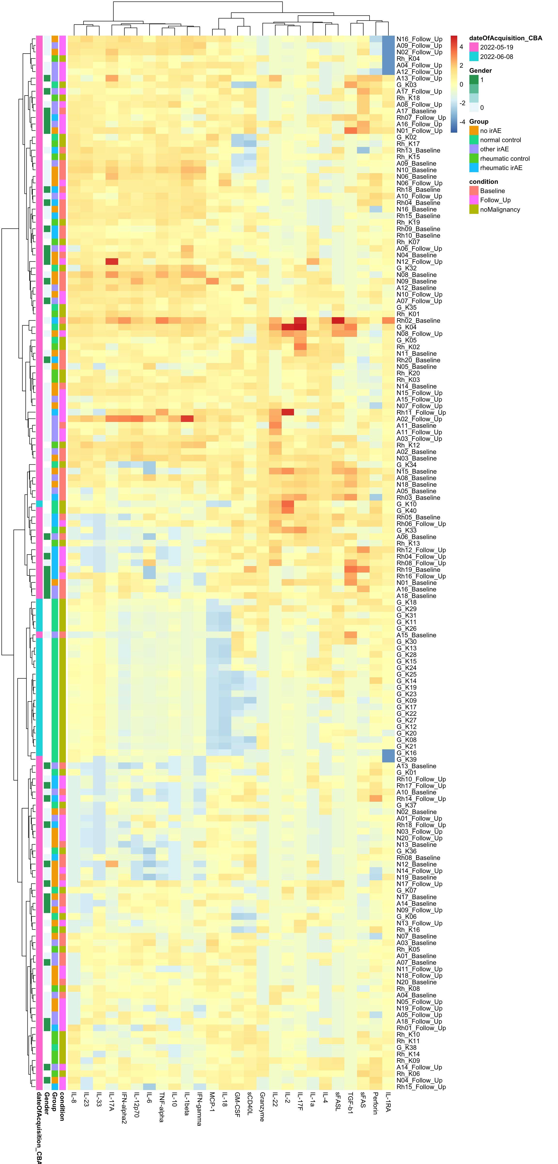
NMR data
Data distribution
Per sample
nmrTab <- filter(fullTab, assay == "NMR")

ggplot(nmrTab, aes(x=sampleID, y=value)) +
    geom_point() +
    theme(axis.text.x = element_text(angle = 90, hjust = 1, vjust = 0.5))
Per feature
ggplot(nmrTab, aes(x=name, y=value)) +
    geom_point() +
    theme(axis.text.x = element_text(angle = 90, hjust = 1, vjust = 0.5))
The data show Heteroskedasticity
###log2 transformation
nmrTab <- mutate(nmrTab, logVal = jyluMisc::glog2(value))
ggplot(nmrTab, aes(x=name, y=logVal)) +
    geom_point() +
    theme(axis.text.x = element_text(angle = 90, hjust = 1, vjust = 0.5))
The log transformation seems not very necessary
PCA
#dataMat <- t(nmrMat)
dataMat <- t(assays(mae)[["nmr"]])
pcRes <- prcomp(dataMat, center = TRUE, scale. = TRUE)
plotTab <- pcRes$x %>% as_tibble(rownames = "sampleID") %>%
    left_join(patAnno, by = "sampleID")

varExp <- pcRes$sdev^2/sum(pcRes$sdev^2)
varTab <- tibble(pc = colnames(pcRes$x), var = varExp*100) %>%
    mutate(pc = factor(pc, levels = pc))
ggplot(varTab, aes(x=pc, y=var)) +
    geom_bar(stat= "identity")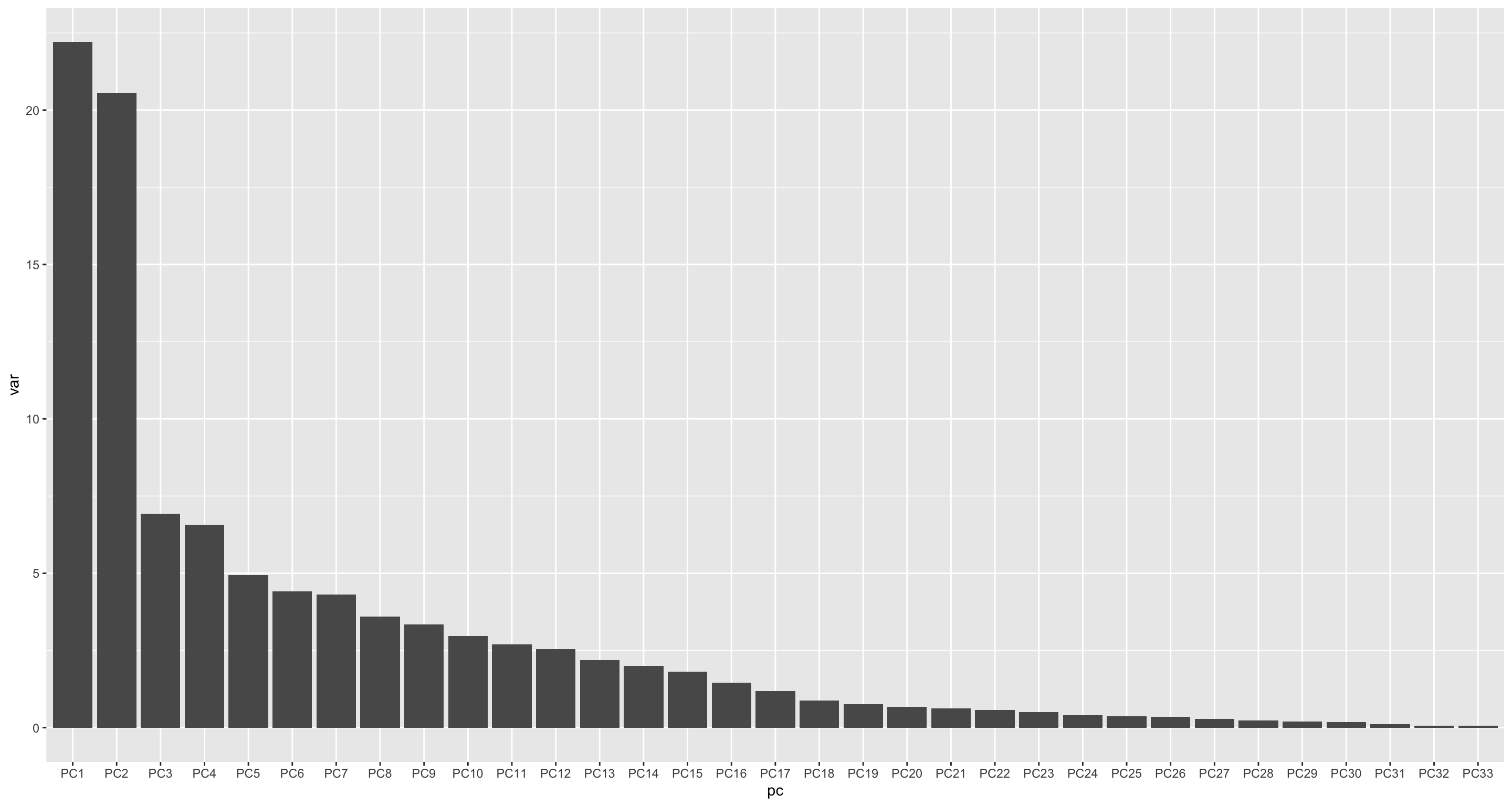
PC1 versus PC2
ggplot(plotTab, aes(x=PC1, y=PC2)) +
    geom_point(aes(color = condition, shape = Group))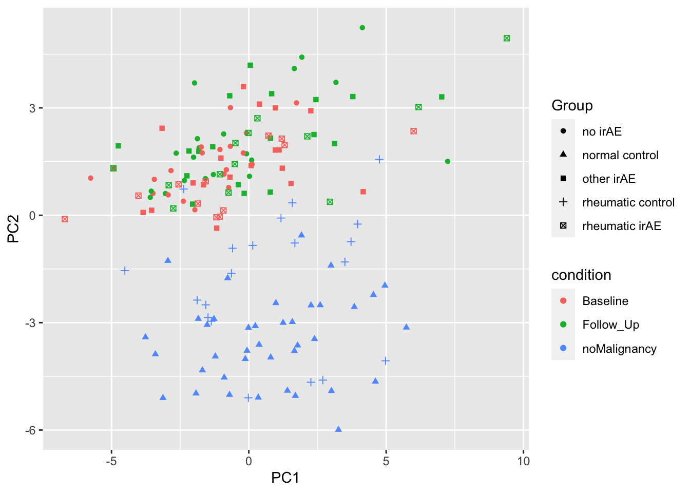
PC3 versus PC4
ggplot(plotTab, aes(x=PC3, y=PC4)) +
    geom_point(aes(color = Group, shape = condition))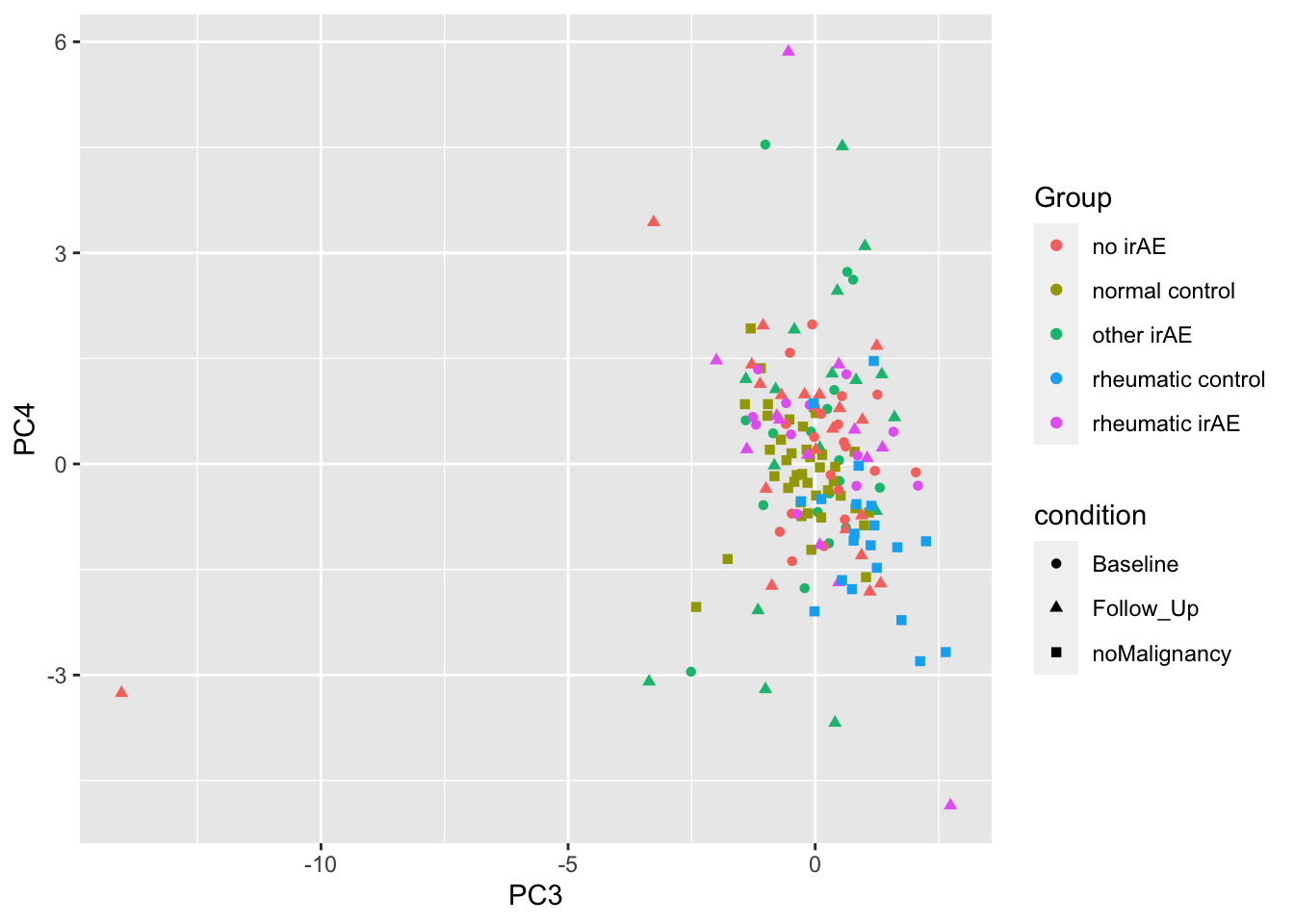
Correlated between PCs and metadata
pcTab <- pcRes$x[,1:20] %>% as_tibble(rownames = "smpID")
metaTab <- colData(mae) %>% as_tibble(rownames = "smpID")
corRes <- jyluMisc::testAssociation(pcTab, metaTab, "smpID")
head(corRes, n=20)
var1 var2 p
1 PC2 Group 6.806470e-47
2 PC2 condition 2.448136e-45
3 PC2 Tumor 2.155078e-42
4 PC2 dateOfAcquisition_NMR 2.974508e-41
5 PC2 dateOfAcquisition_CBA 1.367969e-16
6 PC2 patID 1.832306e-11
7 PC11 patID 2.753020e-07
8 PC7 Date.Sample.Baseline 2.057258e-06
9 PC13 Type.of.irAE 2.262599e-05
10 PC16 Date.Sample.Follow.Up..FU. 2.694168e-05
11 PC7 Date.Sample.Follow.Up..FU. 4.220689e-05
12 PC17 Date.Sample.Baseline 5.811782e-05
13 PC11 Date.Sample.Baseline 5.952632e-05
14 PC17 Date.Sample.Follow.Up..FU. 7.589365e-05
15 PC11 dateOfAcquisition_NMR 1.159803e-04
16 PC12 Gender 1.644228e-04
17 PC12 Height 2.636843e-04
18 PC6 Date.Sample.Follow.Up..FU. 2.768313e-04
19 PC7 patID 3.029784e-04
20 PC4 Date.Sample.Follow.Up..FU. 3.928352e-04ggplot(plotTab, aes(x=PC1, y=PC2)) +
geom_point(aes(color = factor(dateOfAcquisition_NMR), shape = Group), size=3) +
geom_line(aes(group=patID), color = "grey50", linetype = "dotted")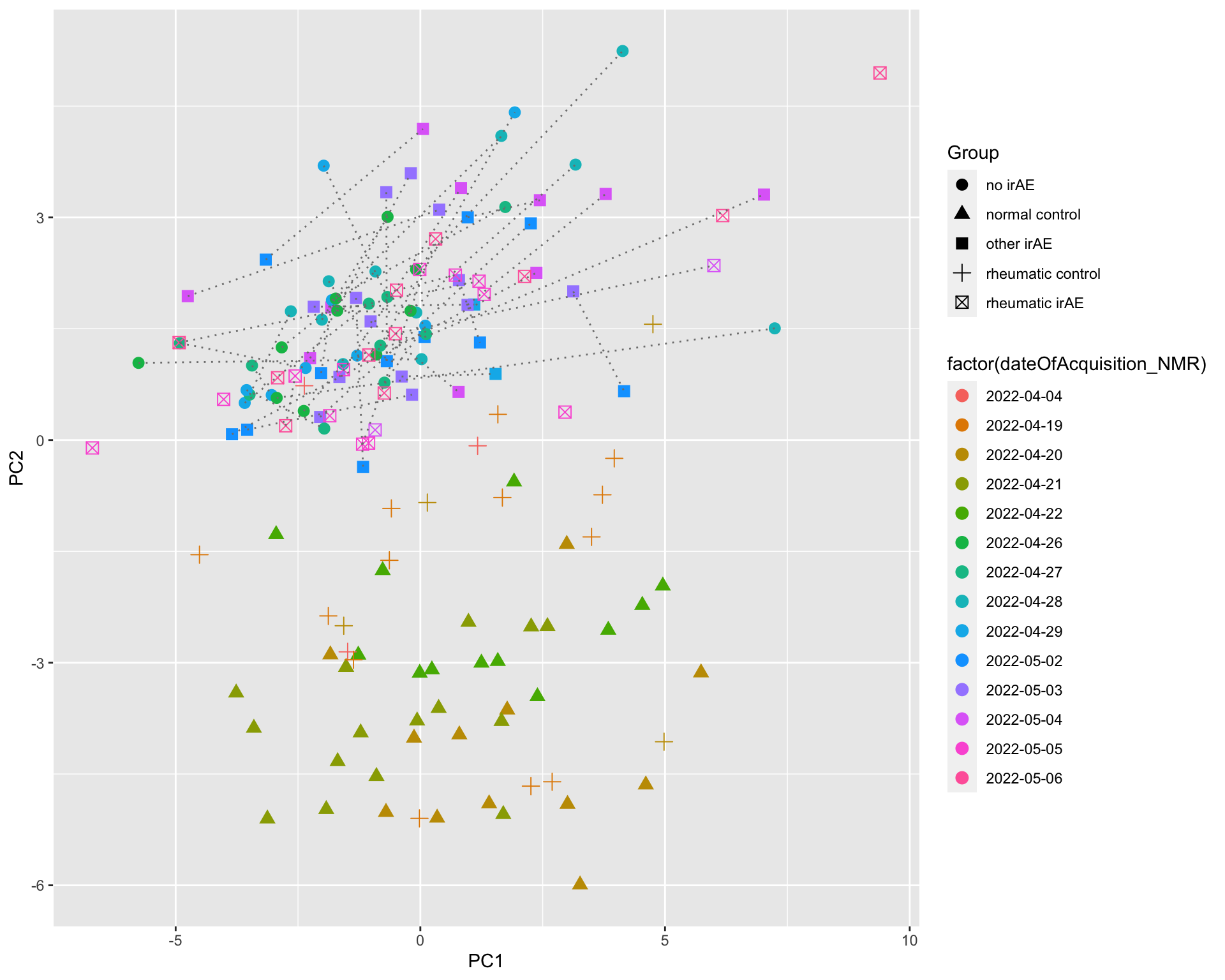
Clustering
annoCol <- colData(mae)[,c("condition","Group","Gender", "dateOfAcquisition_NMR")] %>% data.frame()
annoCol$dateOfAcquisition_NMR <- as.character(annoCol$dateOfAcquisition_NMR)
pheatmap(dataMat, annotation_row = annoCol, clustering_method = "ward.D2")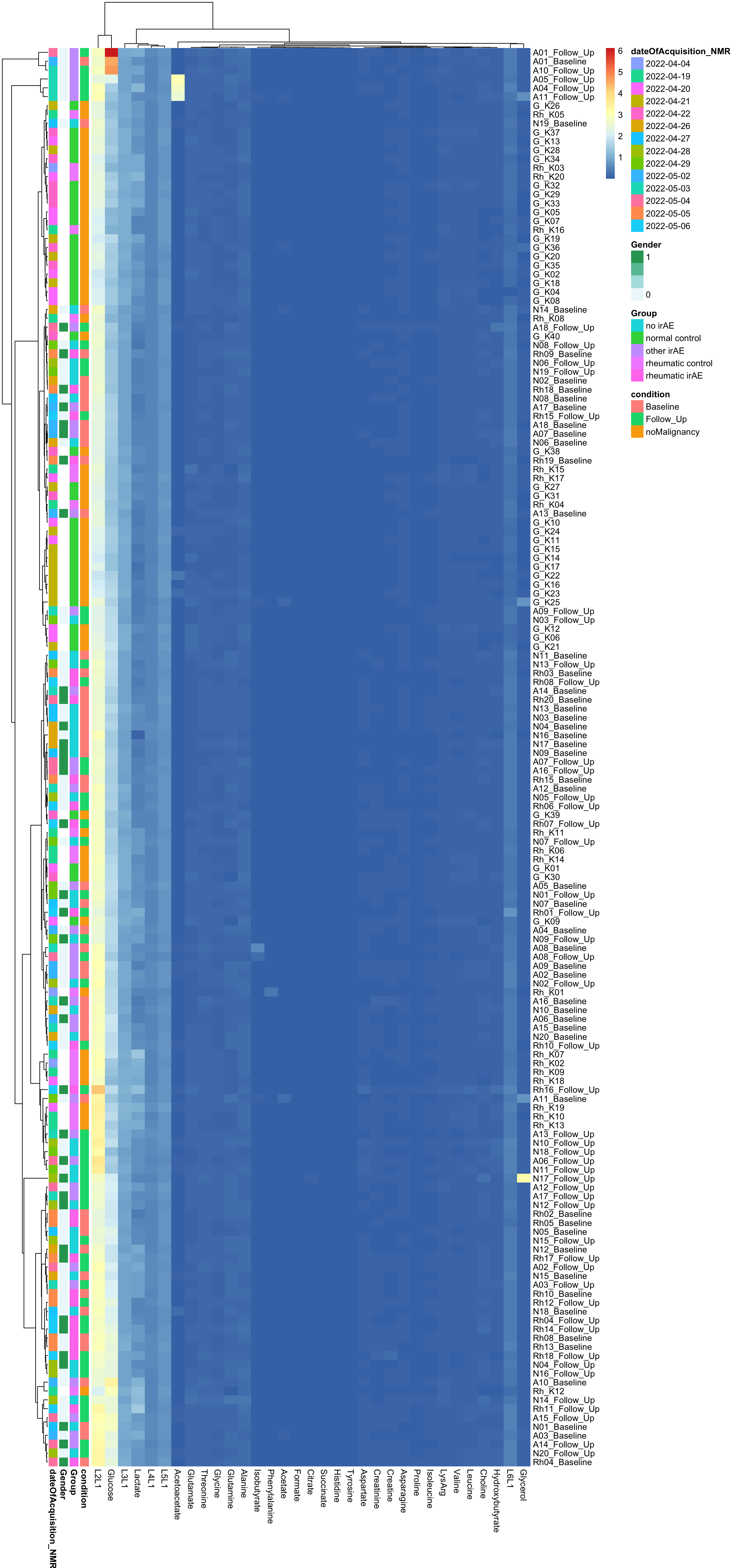
Scaled
pheatmap(dataMat, annotation_row = annoCol, scale="column", clustering_method = "ward.D2")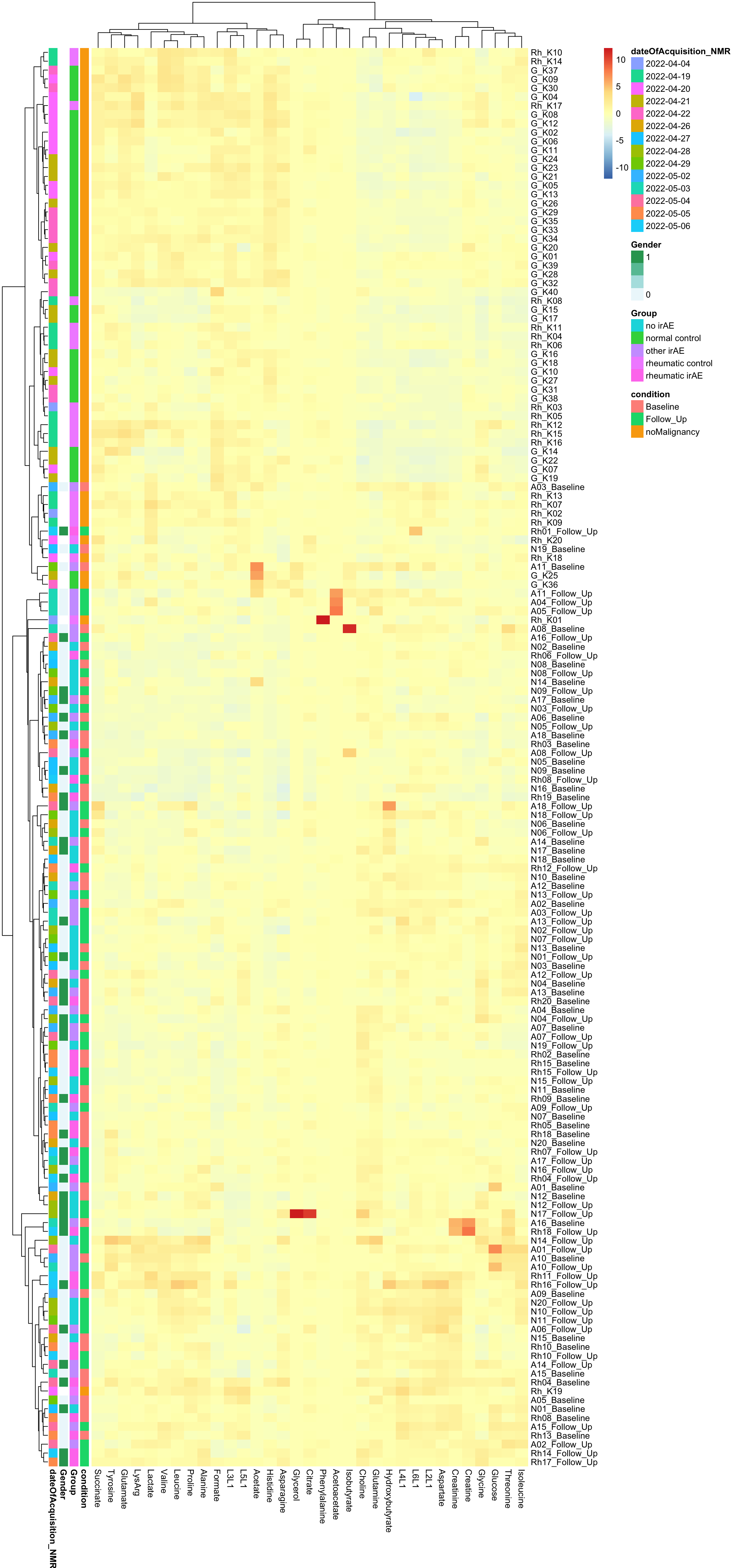
Repeat above analysis without control samples (iRE control and normal control)
Remove control samples
mae <- mae[,mae$condition != "noMalignancy"]CBA data
Data distribution
Per sample
cbaTab <- filter(fullTab, assay == "CBA")

ggplot(cbaTab, aes(x=sampleID, y=value)) +
    geom_point() +
    theme(axis.text.x = element_text(angle = 90, hjust = 1, vjust = 0.5))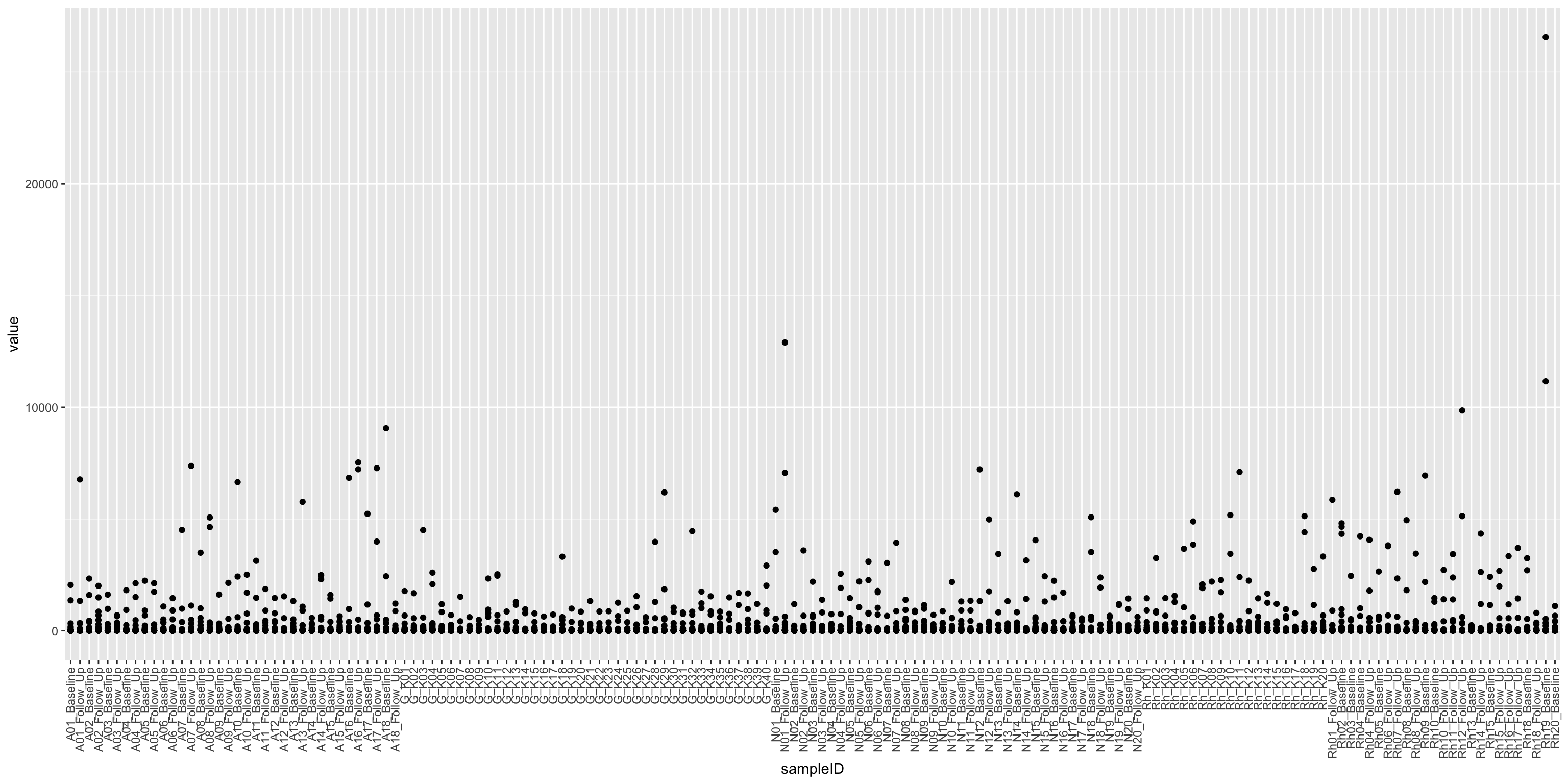
Per feature
ggplot(cbaTab, aes(x=name, y=value)) +
    geom_point() +
    theme(axis.text.x = element_text(angle = 90, hjust = 1, vjust = 0.5))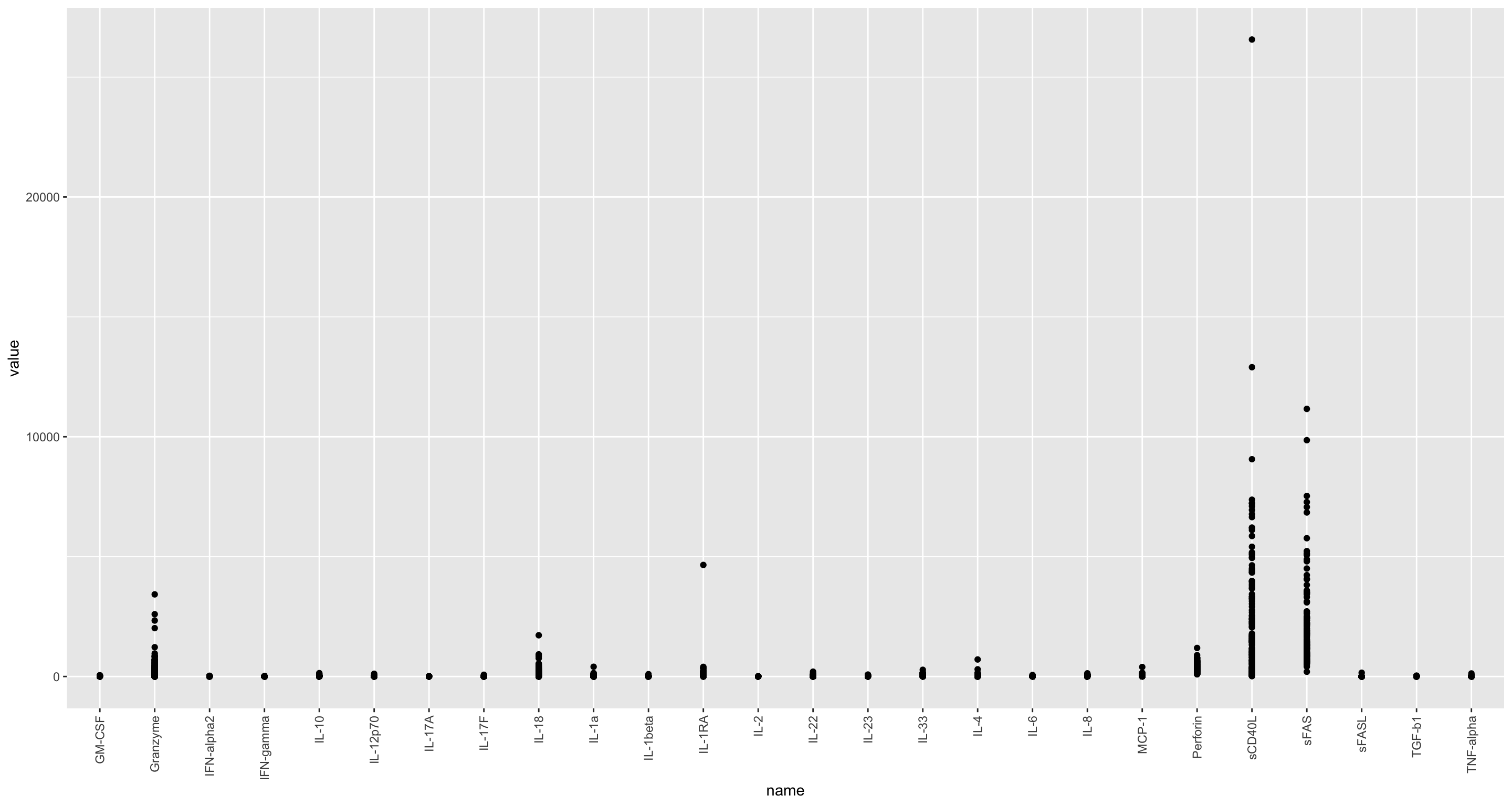
glog2 transformation
cbaTab <- mutate(cbaTab, logVal = jyluMisc::glog2(value))
ggplot(cbaTab, aes(x=name, y=logVal)) +
    geom_point() +
    theme(axis.text.x = element_text(angle = 90, hjust = 1, vjust = 0.5))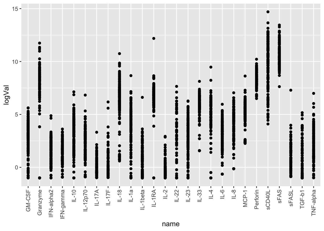
PCA analysis
Use log2 transformed data
Variance explaned
dataMat <- jyluMisc::glog2(t(mae[["cba"]]))
pcRes <- prcomp(dataMat, center = TRUE, scale. = TRUE)
plotTab <- pcRes$x %>% as_tibble(rownames = "sampleID") %>%
    left_join(patAnno, by = "sampleID")

varExp <- pcRes$sdev^2/sum(pcRes$sdev^2)
varTab <- tibble(pc = colnames(pcRes$x), var = varExp*100) %>%
    mutate(pc = factor(pc, levels = pc))
ggplot(varTab, aes(x=pc, y=var)) +
    geom_bar(stat= "identity")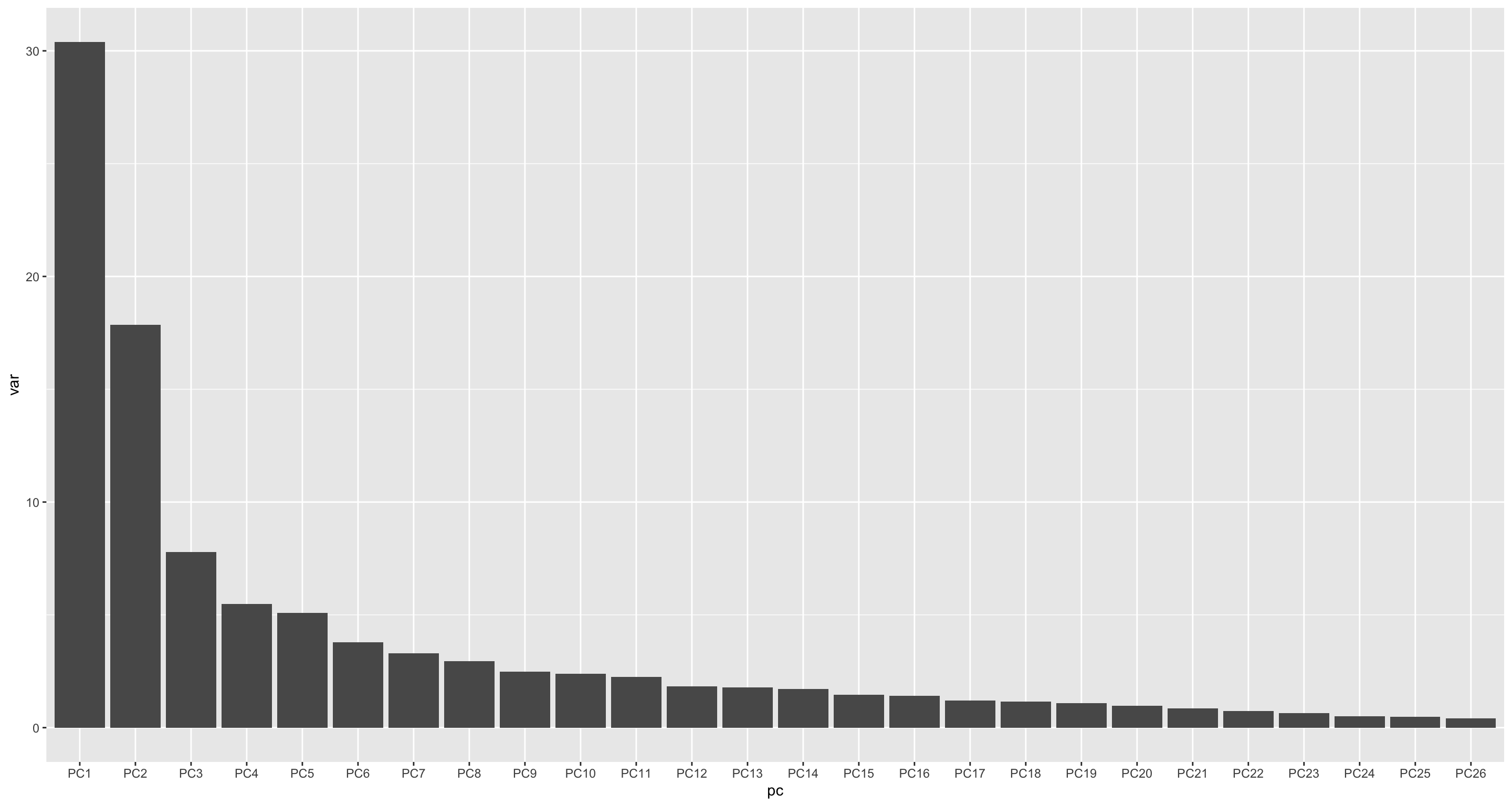
PC1 versus PC2
ggplot(plotTab, aes(x=PC1, y=PC2)) +
    geom_point(aes(color = Group, shape = condition), size=3) +
    geom_line(aes(group=patID), color = "grey50", linetype = "dotted")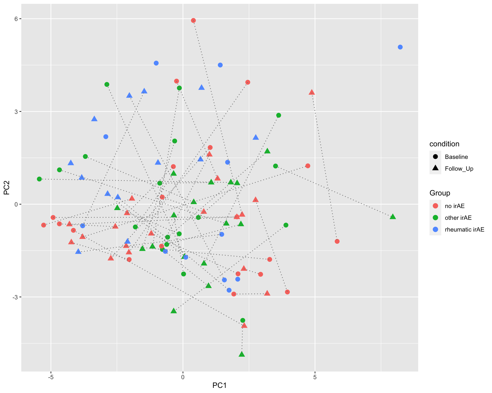
PC3 versus PC4
ggplot(plotTab, aes(x=PC3, y=PC4)) +
    geom_point(aes(color = Group, shape = condition), size=3) +
    geom_line(aes(group=patID), color = "grey50", linetype = "dotted")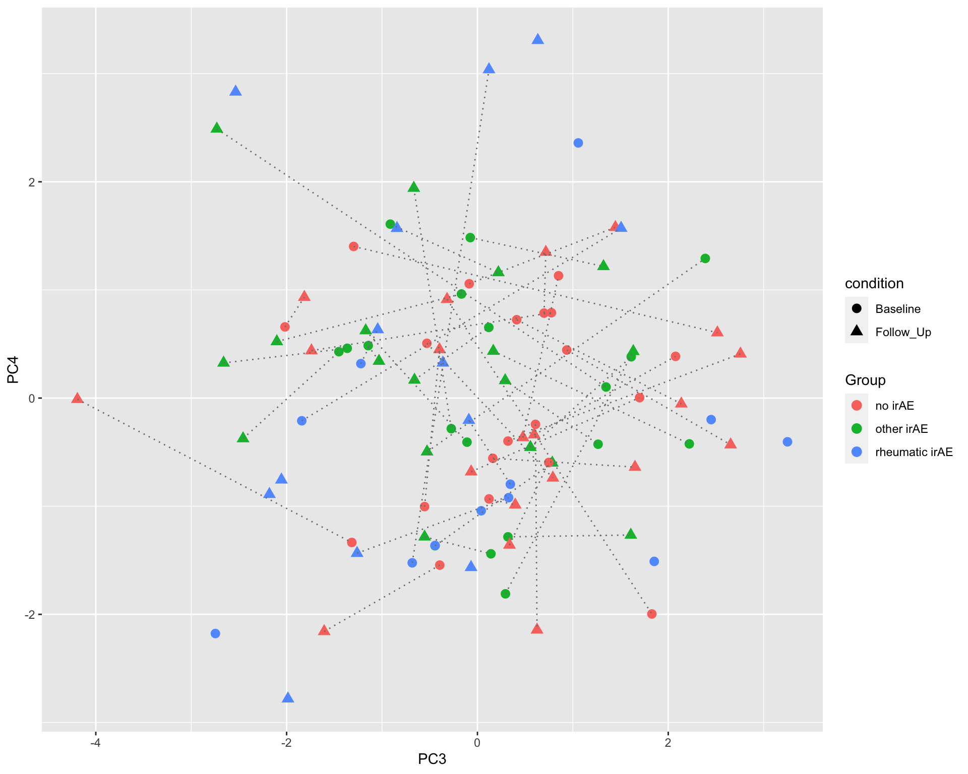
Clustering
Without scaling
annoCol <- colData(mae)[,c("condition","Group","Gender", "dateOfAcquisition_CBA")] %>% data.frame()
annoCol$dateOfAcquisition_CBA <- as.character(annoCol$dateOfAcquisition_CBA)
pheatmap(dataMat, annotation_row = annoCol, clustering_method = "ward.D2")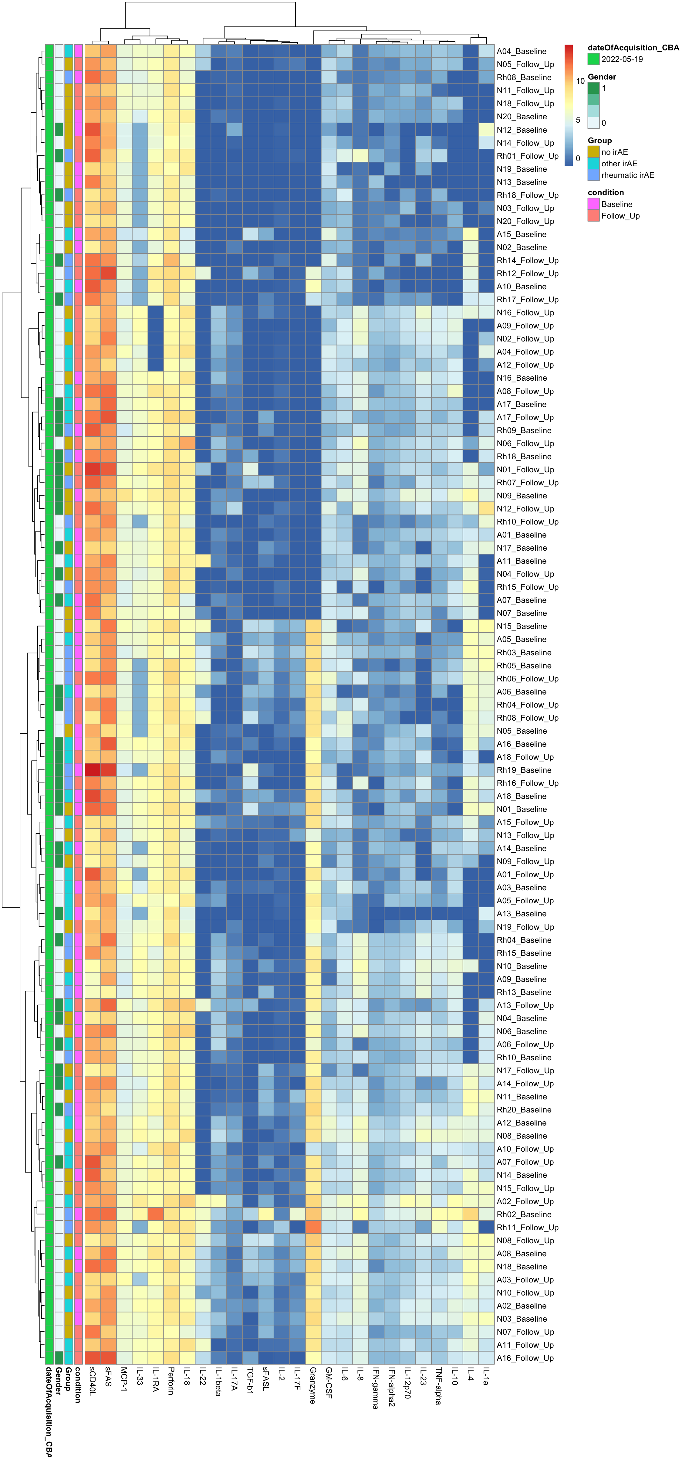
Column Scaled
pheatmap(dataMat, annotation_row = annoCol, scale="column", clustering_method = "ward.D2")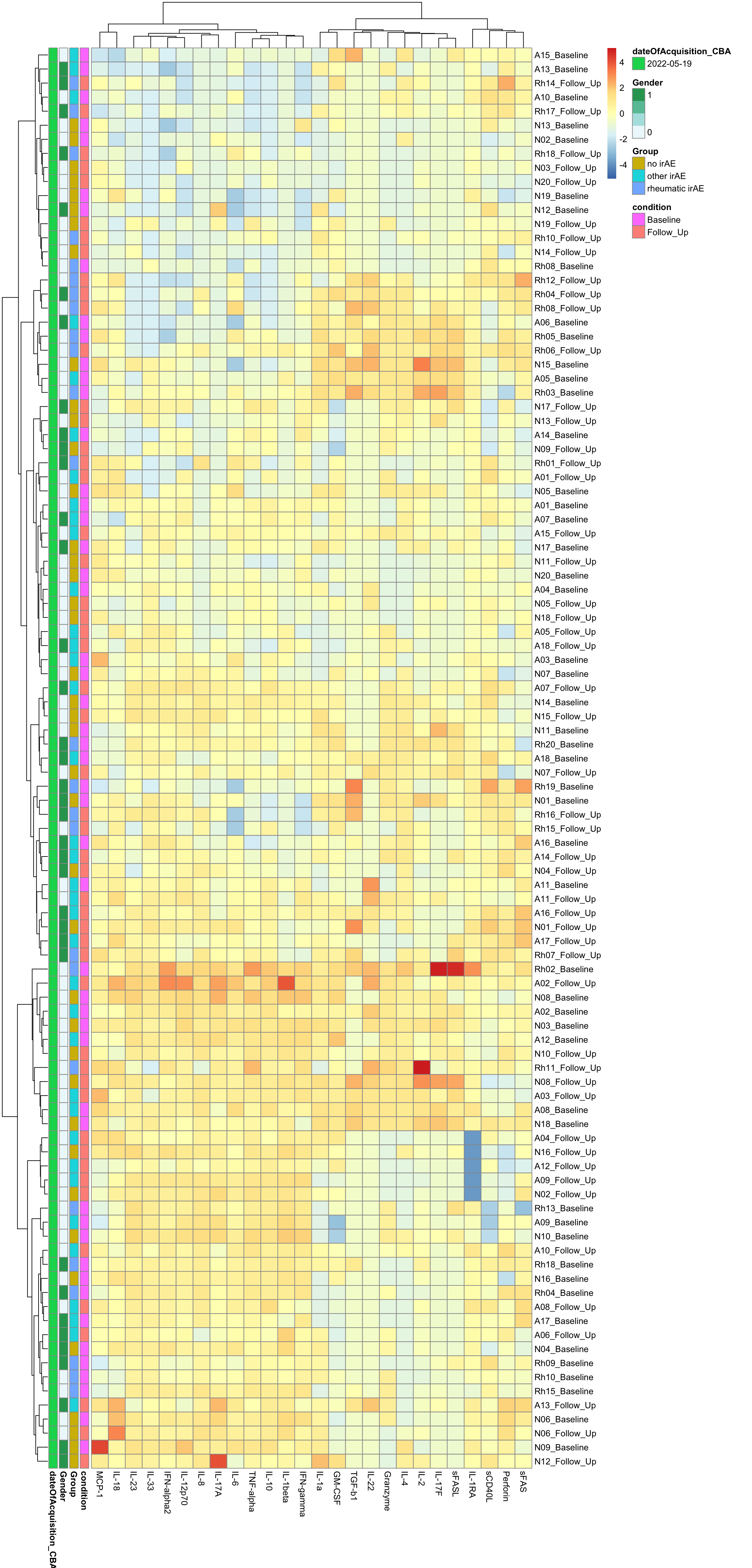
NMR data
Data distribution
Per sample
nmrTab <- filter(fullTab, assay == "NMR")
ggplot(nmrTab, aes(x=sampleID, y=value)) +
geom_point() +
theme(axis.text.x = element_text(angle = 90, hjust = 1, vjust = 0.5))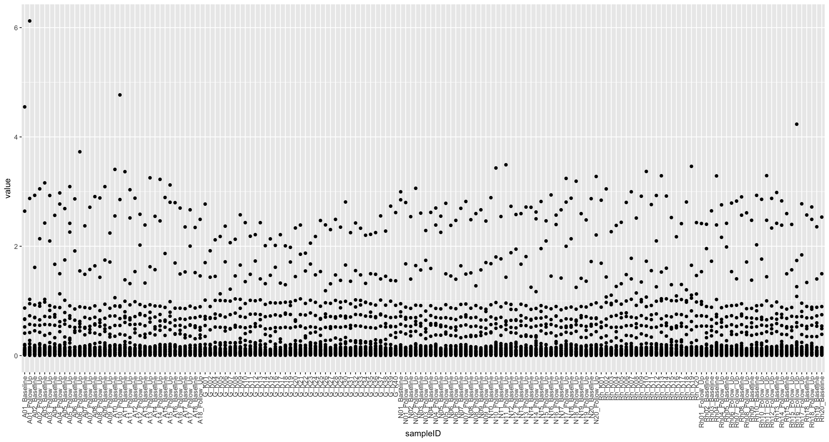
Per feature
ggplot(nmrTab, aes(x=name, y=value)) +
geom_point() +
theme(axis.text.x = element_text(angle = 90, hjust = 1, vjust = 0.5))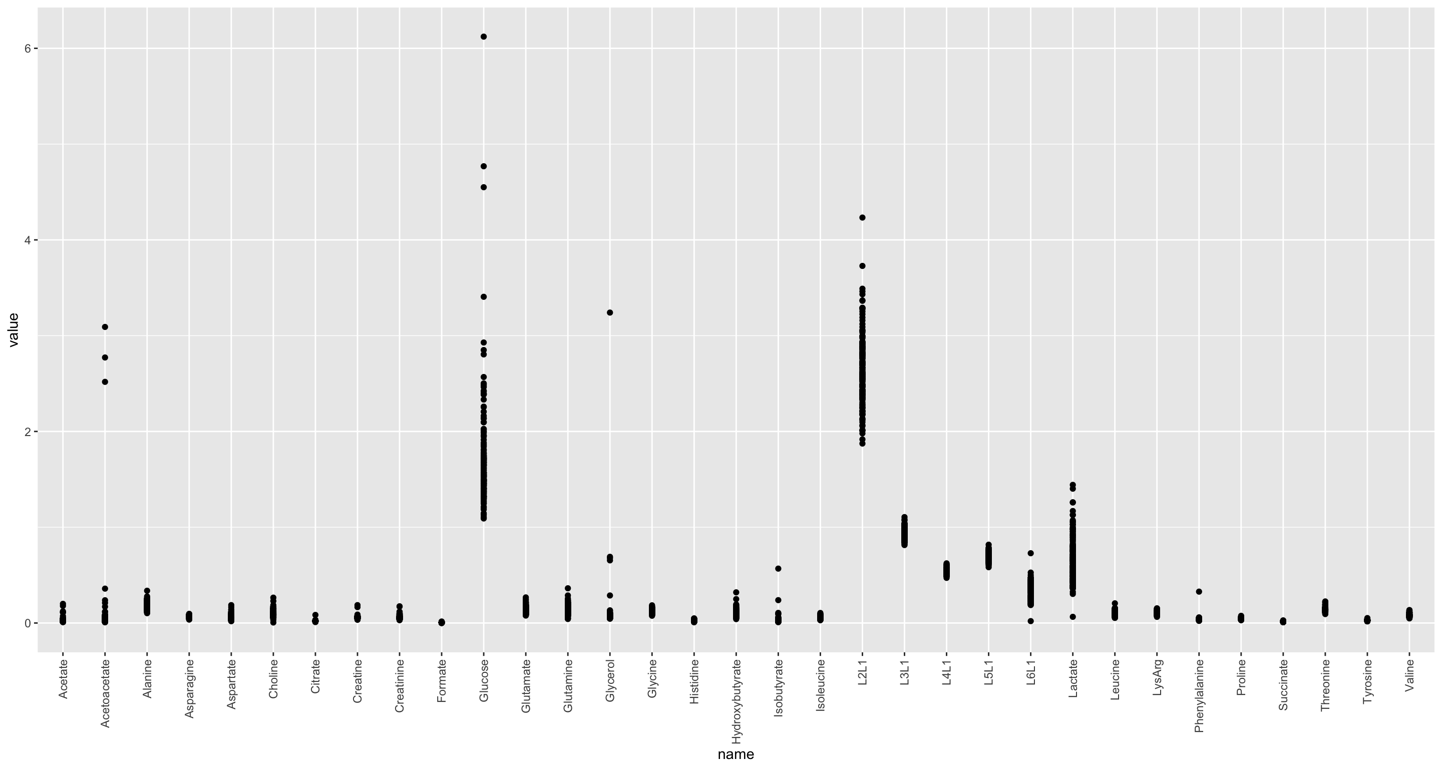 The data show Heteroskedasticity
Need transformation?
nmrTab <- mutate(nmrTab, logVal = jyluMisc::glog2(value))
ggplot(nmrTab, aes(x=name, y=logVal)) +
geom_point() +
theme(axis.text.x = element_text(angle = 90, hjust = 1, vjust = 0.5))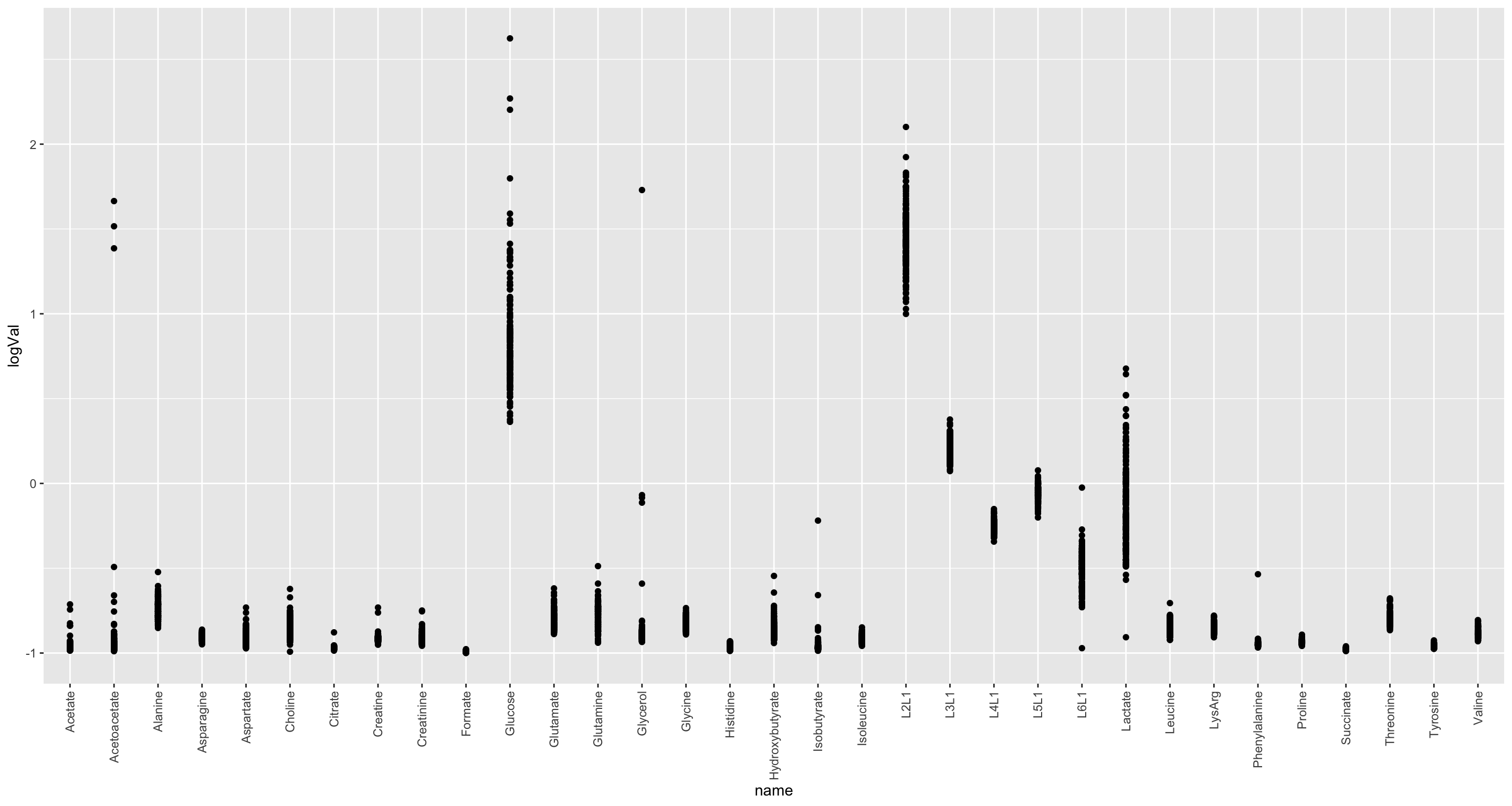 log2 seems not needed
PCA
#dataMat <- t(nmrMat)
dataMat <- t(assays(mae)[["nmr"]])
pcRes <- prcomp(dataMat, center = TRUE, scale. = TRUE)
plotTab <- pcRes$x %>% as_tibble(rownames = "sampleID") %>%
left_join(patAnno, by = "sampleID")
varExp <- pcRes$sdev^2/sum(pcRes$sdev^2)
varTab <- tibble(pc = colnames(pcRes$x), var = varExp*100) %>%
mutate(pc = factor(pc, levels = pc))
ggplot(varTab, aes(x=pc, y=var)) +
geom_bar(stat= "identity")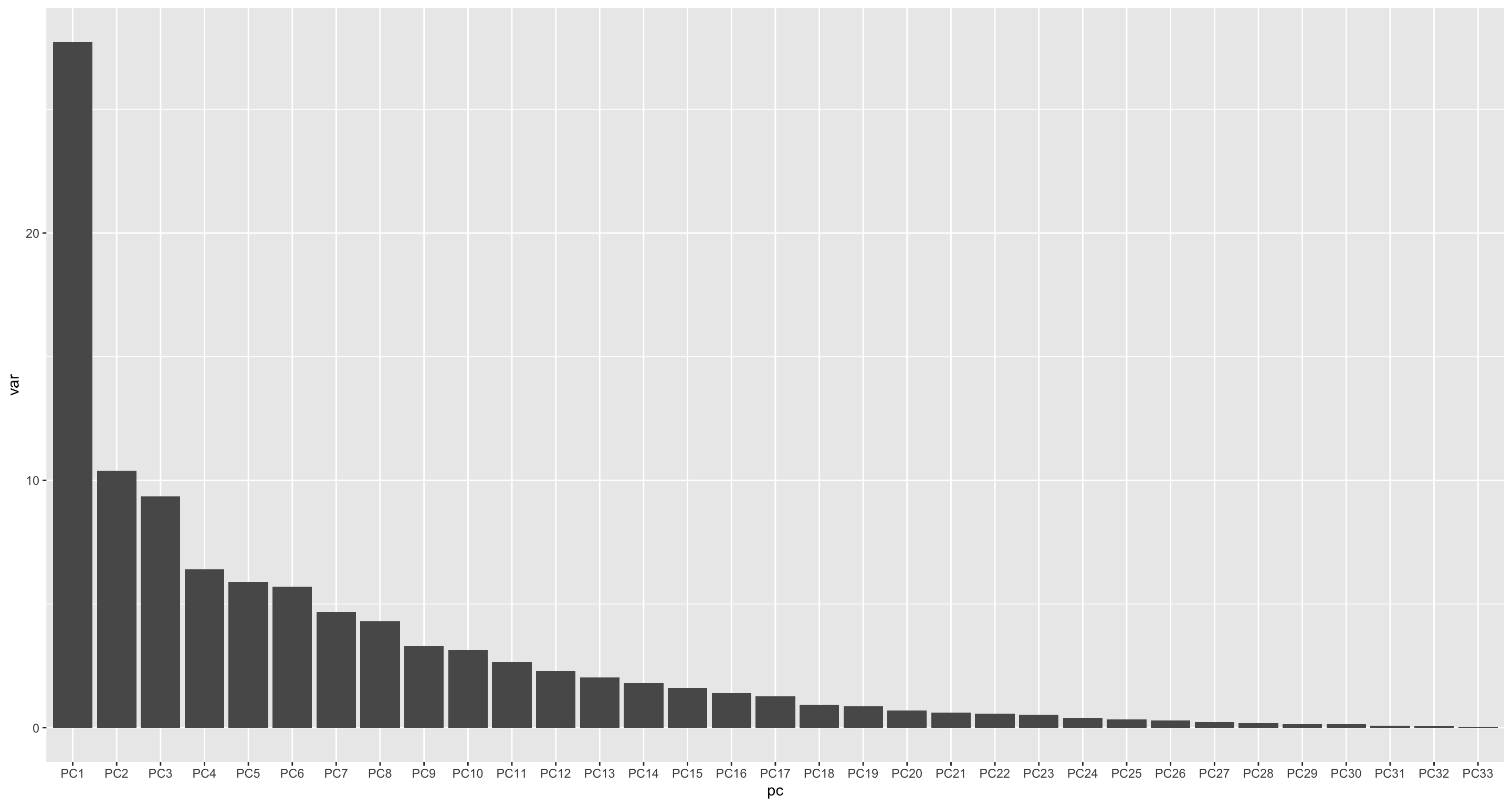
PC1 versus PC2
ggplot(plotTab, aes(x=PC1, y=PC2)) +
geom_point(aes(color = condition, shape = Group))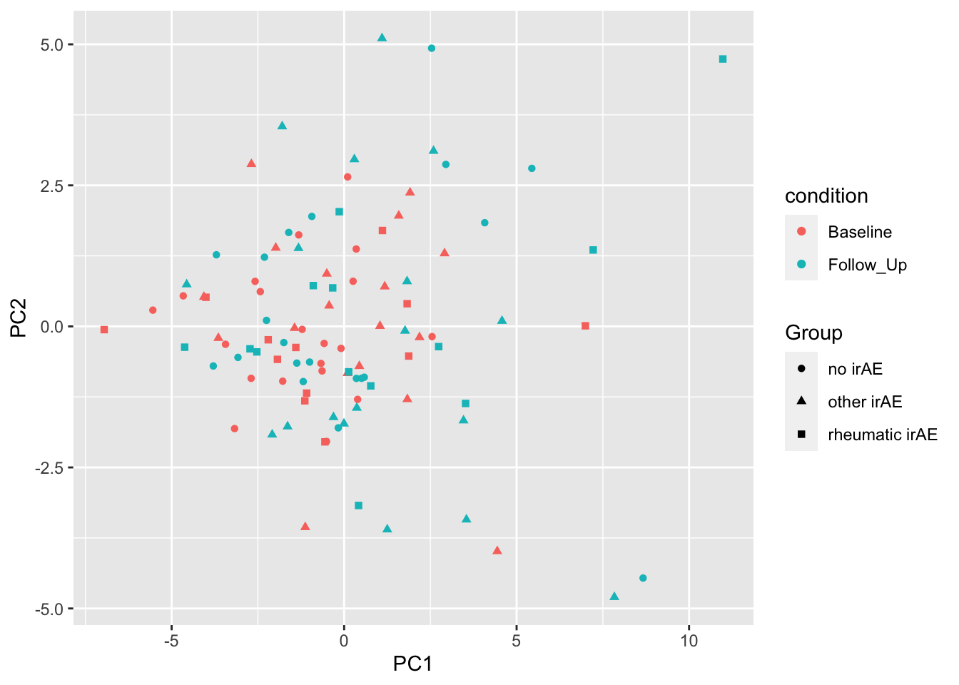
PC3 versus PC4
ggplot(plotTab, aes(x=PC3, y=PC4)) +
geom_point(aes(color = Group, shape = condition))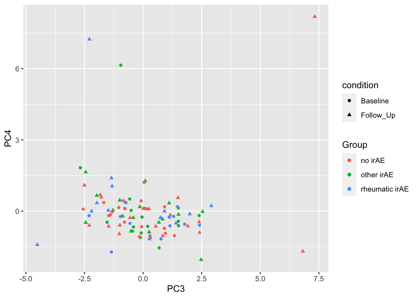
Correlated between PCs and metadata
pcTab <- pcRes$x[,1:20] %>% as_tibble(rownames = "smpID")
metaTab <- colData(mae) %>% as_tibble(rownames = "smpID")
corRes <- jyluMisc::testAssociation(pcTab, metaTab, "smpID")
head(corRes, n=20)
var1 var2 p
1 PC13 Group 1.004989e-06
2 PC5 patID 2.680285e-06
3 PC9 Date.Sample.Follow.Up..FU. 4.055509e-06
4 PC5 Date.Sample.Follow.Up..FU. 1.153460e-05
5 PC16 Rheumatoid.Factor 3.230266e-05
6 PC10 Height 3.622505e-05
7 PC9 Type.of.irAE 9.050051e-05
8 PC10 Gender 1.024334e-04
9 PC13 dateOfAcquisition_NMR 1.102883e-04
10 PC13 patID 1.497625e-04
11 PC11 ANA 1.554890e-04
12 PC13 Date.Sample.Follow.Up..FU. 1.660475e-04
13 PC17 Last.staging.before.FU 1.712301e-04
14 PC9 patID 1.805000e-04
15 PC5 Date.Sample.Baseline 1.811005e-04
16 PC9 Date.Sample.Baseline 2.330708e-04
17 PC20 Weight.at.Baseline 2.580965e-04
18 PC3 ICI.Duration 2.713748e-04
19 PC16 patID 5.365390e-04
20 PC13 Type.of.irAE 7.210380e-04ggplot(plotTab, aes(x=PC8, y=PC19)) +
geom_point(aes(color = factor(Gender), shape = Group), size=3) +
geom_line(aes(group=patID), color = "grey50", linetype = "dotted")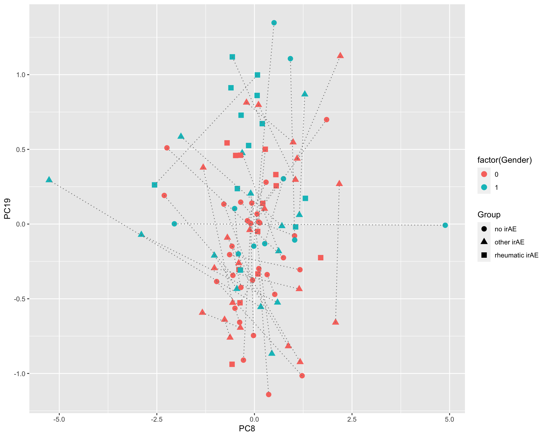
Clustering
annoCol <- colData(mae)[,c("condition","Group","Gender", "dateOfAcquisition_NMR")] %>% data.frame()
annoCol$dateOfAcquisition_NMR <- as.character(annoCol$dateOfAcquisition_NMR)
pheatmap(dataMat, annotation_row = annoCol, clustering_method = "ward.D2")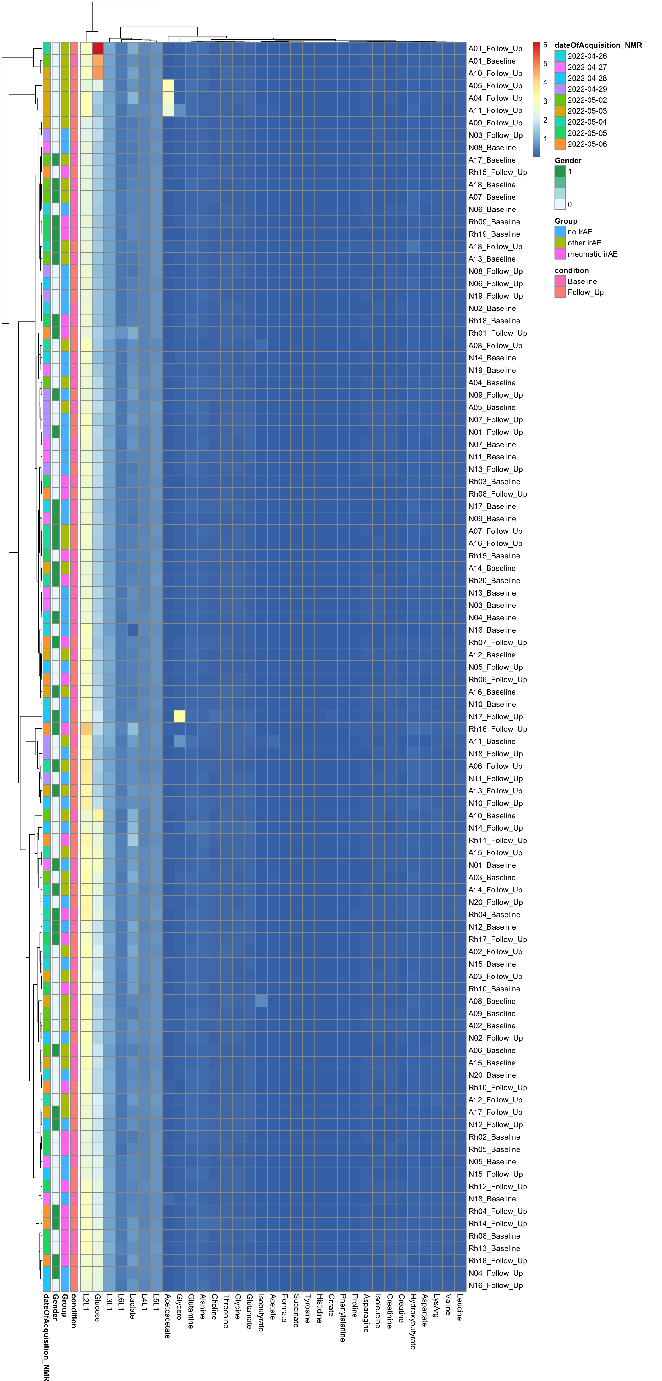
Scaled
pheatmap(dataMat, annotation_row = annoCol, scale="column", clustering_method = "ward.D2")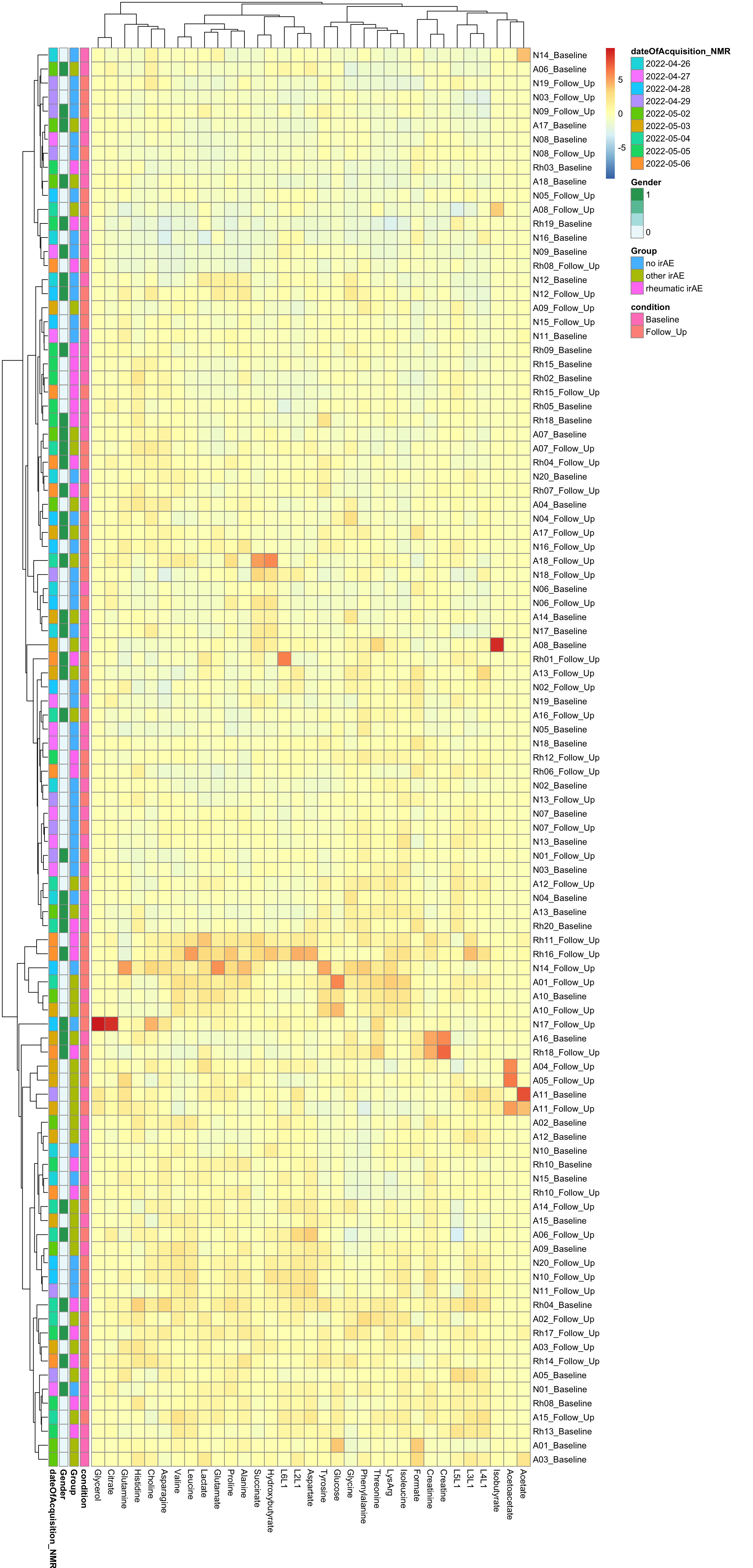
sessionInfo()R version 4.2.0 (2022-04-22)
Platform: x86_64-apple-darwin17.0 (64-bit)
Running under: macOS Big Sur/Monterey 10.16
Matrix products: default
BLAS: /Library/Frameworks/R.framework/Versions/4.2/Resources/lib/libRblas.0.dylib
LAPACK: /Library/Frameworks/R.framework/Versions/4.2/Resources/lib/libRlapack.dylib
locale:
[1] en_US.UTF-8/en_US.UTF-8/en_US.UTF-8/C/en_US.UTF-8/en_US.UTF-8
attached base packages:
[1] stats4 stats graphics grDevices utils datasets methods
[8] base
other attached packages:
[1] forcats_0.5.1 stringr_1.4.0
[3] dplyr_1.0.9 purrr_0.3.4
[5] readr_2.1.2 tidyr_1.2.0
[7] tibble_3.1.8 ggplot2_3.3.6
[9] tidyverse_1.3.2 vsn_3.64.0
[11] pheatmap_1.0.12 MultiAssayExperiment_1.22.0
[13] SummarizedExperiment_1.26.1 Biobase_2.56.0
[15] GenomicRanges_1.48.0 GenomeInfoDb_1.32.2
[17] IRanges_2.30.0 S4Vectors_0.34.0
[19] BiocGenerics_0.42.0 MatrixGenerics_1.8.1
[21] matrixStats_0.62.0
loaded via a namespace (and not attached):
[1] readxl_1.4.0 backports_1.4.1 fastmatch_1.1-3
[4] drc_3.0-1 jyluMisc_0.1.5 workflowr_1.7.0
[7] igraph_1.3.4 shinydashboard_0.7.2 splines_4.2.0
[10] BiocParallel_1.30.3 TH.data_1.1-1 digest_0.6.29
[13] htmltools_0.5.3 fansi_1.0.3 magrittr_2.0.3
[16] googlesheets4_1.0.0 cluster_2.1.3 tzdb_0.3.0
[19] limma_3.52.2 modelr_0.1.8 sandwich_3.0-2
[22] piano_2.12.0 colorspace_2.0-3 rvest_1.0.2
[25] haven_2.5.0 xfun_0.31 crayon_1.5.1
[28] RCurl_1.98-1.7 jsonlite_1.8.0 survival_3.4-0
[31] zoo_1.8-10 glue_1.6.2 survminer_0.4.9
[34] gtable_0.3.0 gargle_1.2.0 zlibbioc_1.42.0
[37] XVector_0.36.0 DelayedArray_0.22.0 car_3.1-0
[40] abind_1.4-5 scales_1.2.0 mvtnorm_1.1-3
[43] DBI_1.1.3 relations_0.6-12 rstatix_0.7.0
[46] Rcpp_1.0.9 plotrix_3.8-2 xtable_1.8-4
[49] km.ci_0.5-6 preprocessCore_1.58.0 DT_0.23
[52] htmlwidgets_1.5.4 httr_1.4.3 fgsea_1.22.0
[55] gplots_3.1.3 RColorBrewer_1.1-3 ellipsis_0.3.2
[58] pkgconfig_2.0.3 farver_2.1.1 sass_0.4.2
[61] dbplyr_2.2.1 utf8_1.2.2 tidyselect_1.1.2
[64] labeling_0.4.2 rlang_1.0.4 later_1.3.0
[67] visNetwork_2.1.0 munsell_0.5.0 cellranger_1.1.0
[70] tools_4.2.0 cachem_1.0.6 cli_3.3.0
[73] generics_0.1.3 broom_1.0.0 evaluate_0.15
[76] fastmap_1.1.0 yaml_2.3.5 knitr_1.39
[79] fs_1.5.2 survMisc_0.5.6 caTools_1.18.2
[82] mime_0.12 slam_0.1-50 xml2_1.3.3
[85] compiler_4.2.0 rstudioapi_0.13 ggsignif_0.6.3
[88] affyio_1.66.0 marray_1.74.0 reprex_2.0.1
[91] bslib_0.4.0 stringi_1.7.8 highr_0.9
[94] lattice_0.20-45 Matrix_1.4-1 KMsurv_0.1-5
[97] shinyjs_2.1.0 vctrs_0.4.1 pillar_1.8.0
[100] lifecycle_1.0.1 BiocManager_1.30.18 jquerylib_0.1.4
[103] data.table_1.14.2 cowplot_1.1.1 bitops_1.0-7
[106] httpuv_1.6.5 R6_2.5.1 affy_1.74.0
[109] promises_1.2.0.1 KernSmooth_2.23-20 gridExtra_2.3
[112] codetools_0.2-18 MASS_7.3-58 gtools_3.9.3
[115] exactRankTests_0.8-35 assertthat_0.2.1 rprojroot_2.0.3
[118] withr_2.5.0 multcomp_1.4-19 GenomeInfoDbData_1.2.8
[121] parallel_4.2.0 hms_1.1.1 grid_4.2.0
[124] rmarkdown_2.14 carData_3.0-5 googledrive_2.0.0
[127] ggpubr_0.4.0 git2r_0.30.1 maxstat_0.7-25
[130] sets_1.0-21 shiny_1.7.2 lubridate_1.8.0