Last updated: 2022-11-11

Checks: 5 1

Knit directory: irAE_LungCancer/analysis/

This reproducible R Markdown analysis was created with workflowr (version 1.7.0). The Checks tab describes the reproducibility checks that were applied when the results were created. The Past versions tab lists the development history.

Environment: empty

Great job! The global environment was empty. Objects defined in the global environment can affect the analysis in your R Markdown file in unknown ways. For reproduciblity it’s best to always run the code in an empty environment.

Seed: set.seed(20221110)

The command set.seed(20221110) was run prior to running the code in the R Markdown file. Setting a seed ensures that any results that rely on randomness, e.g. subsampling or permutations, are reproducible.

Session information: recorded

Great job! Recording the operating system, R version, and package versions is critical for reproducibility.

Cache: none

Nice! There were no cached chunks for this analysis, so you can be confident that you successfully produced the results during this run.

File paths: relative

Great job! Using relative paths to the files within your workflowr project makes it easier to run your code on other machines.

Repository version: no version control

Tracking code development and connecting the code version to the results is critical for reproducibility. To start using Git, open the Terminal and type git init in your project directory.

This project is not being versioned with Git. To obtain the full reproducibility benefits of using workflowr, please see ?wflow_start.

Load packages

library(MultiAssayExperiment)
library(pheatmap)
library(vsn)
library(jyluMisc)
library(tidyverse)

knitr::opts_chunk$set(warning = FALSE, message = FALSE)

Load data

load("../output/processedData.RData")
patAnno <- colData(mae) %>%
    as_tibble(rownames = "sampleID")

Analyses focused on cancer patients

CBA data

cbaTab <- filter(fullTab, assay == "CBA") %>%
    mutate(logVal = glog2(value)) %>%
    mutate(Group = factor(Group, levels = c("no irAE","rheumatic irAE","other irAE")))

Baseline samples

subTab <- filter(cbaTab, condition == "Baseline" )

PCA

subMat <- subTab %>% select(sampleID, name, logVal) %>%
    pivot_wider(names_from = name, values_from = logVal) %>%
    column_to_rownames("sampleID") %>% as.matrix()

pcRes <- prcomp(subMat, center = TRUE, scale. = TRUE)
pcTab <- pcRes$x %>% as_tibble(rownames = "sampleID") %>%
    left_join(patAnno, by = "sampleID")

ggplot(pcTab, aes(x=PC1, y=PC2, col = Group)) +
    geom_point()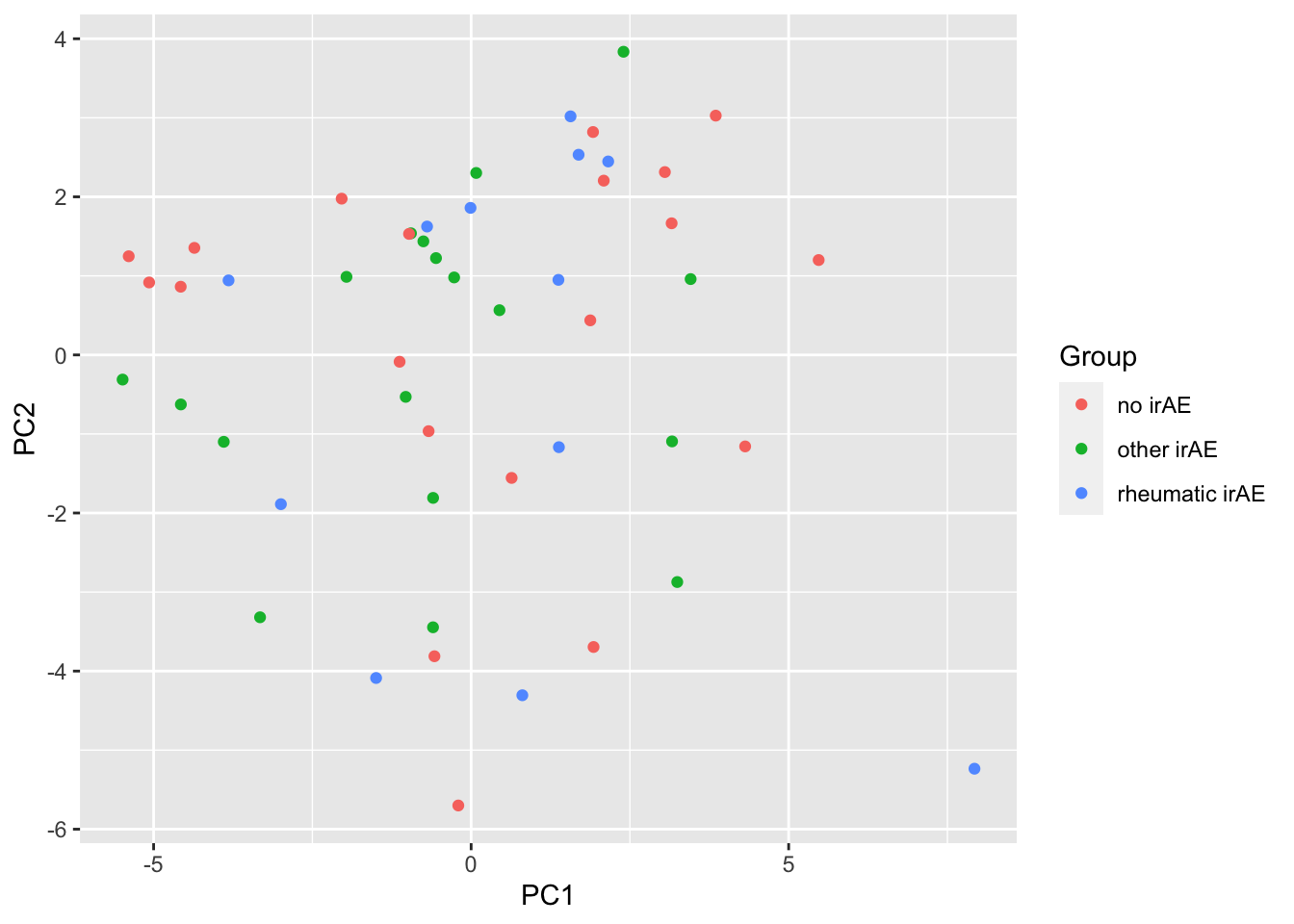

ggplot(pcTab, aes(x=PC3, y=PC4, col = Group)) +
    geom_point()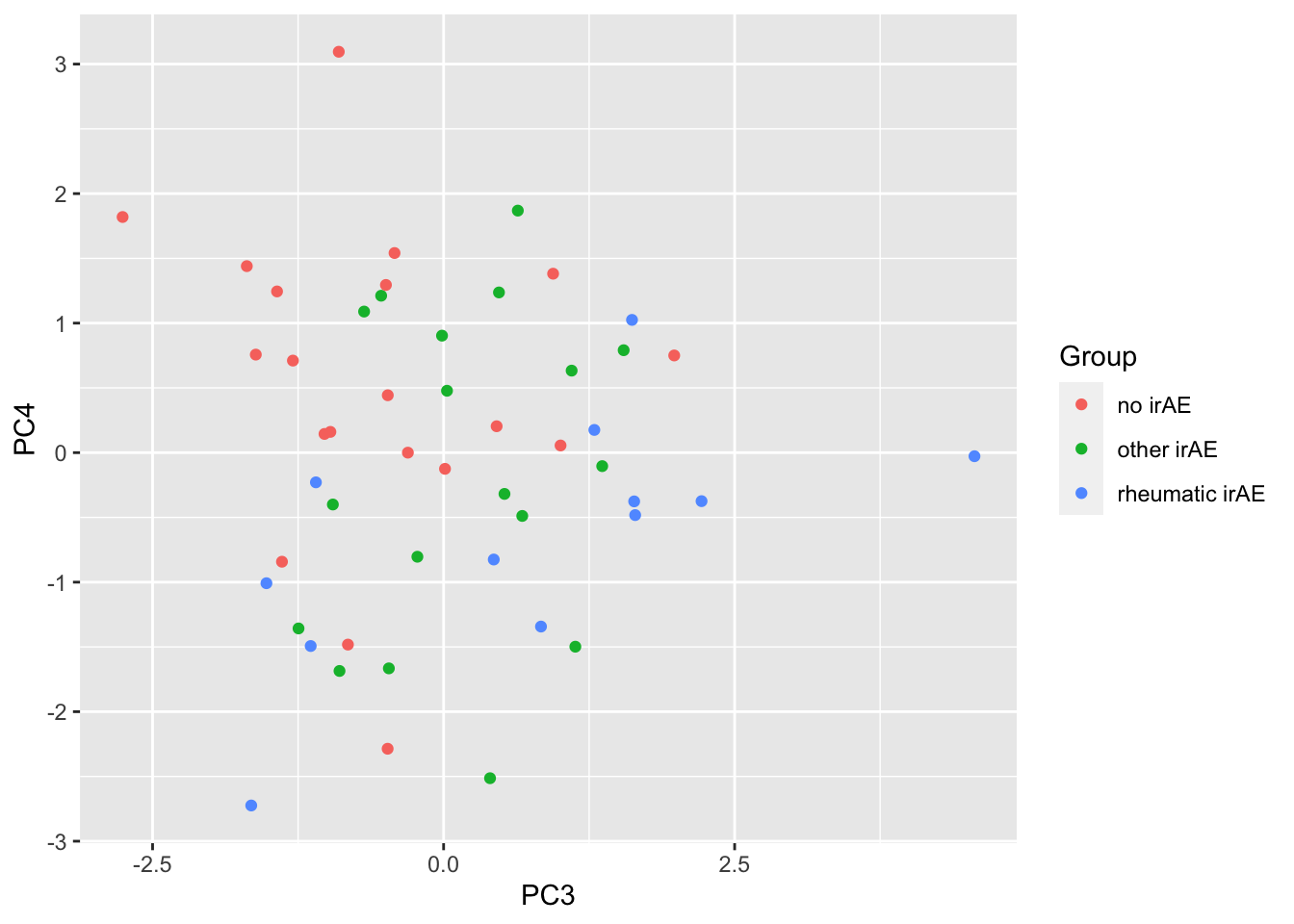

Any PC separate different group?

testTab <- pcTab %>% select(sampleID, PC1:PC20, Group) %>%
    pivot_longer(-c(sampleID, Group)) 
resTab <- group_by(testTab, name) %>% nest() %>%
    mutate(m = map(data, ~aov(lm(value ~ Group,.)))) %>%
    mutate(res = map(m, broom::tidy)) %>%
    unnest(res) %>%
    filter(term == "Group") %>% arrange(p.value)
resTab %>% select(name, p.value) %>% filter(p.value <=0.05)

# A tibble: 2 × 2
# Groups:   name [2]
  name  p.value
  <chr>   <dbl>
1 PC3    0.0162
2 PC4    0.0267

PC3 versus PC4

ggplot(pcTab, aes(x=PC3, y=PC4, col = Group)) +
    geom_point()

ANOVA test

resTab <- subTab %>% group_by(name) %>% nest() %>%
    mutate(m = map(data, ~aov(lm(logVal ~ Group,.)))) %>%
    mutate(res = map(m, broom::tidy)) %>%
    unnest(res) %>%
    filter(term == "Group") %>%
    arrange(p.value) %>%
    select(name, p.value)
resTab.sig <- filter(resTab, p.value < 0.05)
resTab.sig

# A tibble: 1 × 2
# Groups:   name [1]
  name  p.value
  <chr>   <dbl>
1 MCP-1  0.0163

Plot

plotTab <- filter(subTab, name %in% resTab.sig$name)
ggplot(plotTab, aes(x=Group, y=logVal)) +
    geom_boxplot() + geom_point() +
    facet_wrap(~name, scales = "free")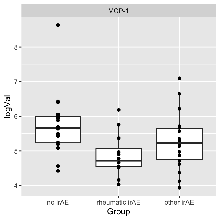

Pair-wise comparison between phenotypes

pairwiseT <- function(dataTab, value, group, feature) {
    if (is.factor(dataTab[[group]])) {
         allCompare <- combn(levels(dataTab[[group]]),2, simplify = FALSE)
    } else {
        allCompare <- combn(unique(dataTab[[group]]),2, simplify = FALSE)
    }
    testTab <- select(dataTab, all_of(c(value, group, feature))) %>%
        dplyr::rename(group = all_of(group), 
                      value = all_of(value),
                      feature = all_of(feature)) 
    resTab <- lapply(allCompare, function(x) {
        refGroup <- x[1]
        comGroup <- x[2]
        eachTab <- filter(testTab, group %in% c(refGroup, comGroup)) %>%
            mutate(group = factor(group, levels = c(refGroup, comGroup)))
        res <- group_by(eachTab, feature) %>% nest() %>%
            mutate(m = map(data, ~t.test(value~group,.,var.equal=TRUE))) %>%
            mutate(r = map(m, broom::tidy)) %>% unnest(r) %>%
            select(feature, estimate, p.value) %>%
            mutate(group1 = refGroup, group2 = comGroup) %>%
            arrange(p.value) %>% ungroup() %>%
            mutate(p.adj = p.adjust(p.value, method = "BH"))
        
    }) %>% bind_rows() 
}

resPair.baseline <- pairwiseT(subTab, "logVal", "Group", "name")
filter(resPair.baseline, p.value < 0.05)

# A tibble: 4 × 6
  feature   estimate p.value group1         group2         p.adj
  <chr>        <dbl>   <dbl> <chr>          <chr>          <dbl>
1 MCP-1        0.861 0.00563 no irAE        rheumatic irAE 0.146
2 IL-18        0.824 0.0381  no irAE        other irAE     0.514
3 IL-17A       0.526 0.0444  no irAE        other irAE     0.514
4 TNF-alpha    1.22  0.0496  rheumatic irAE other irAE     0.701

Follow-up samples

subTab <- filter(cbaTab, condition == "Follow_Up" )

PCA

subMat <- subTab %>% select(sampleID, name, logVal) %>%
    pivot_wider(names_from = name, values_from = logVal) %>%
    column_to_rownames("sampleID") %>% as.matrix()

pcRes <- prcomp(subMat, center = TRUE, scale. = TRUE)
pcTab <- pcRes$x %>% as_tibble(rownames = "sampleID") %>%
    left_join(patAnno, by = "sampleID")

ggplot(pcTab, aes(x=PC1, y=PC2, col = Group)) +
    geom_point()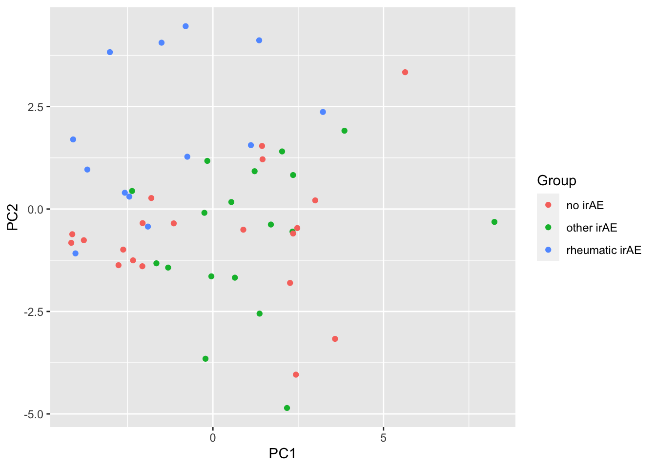

ggplot(pcTab, aes(x=PC3, y=PC4, col = Group)) +
    geom_point()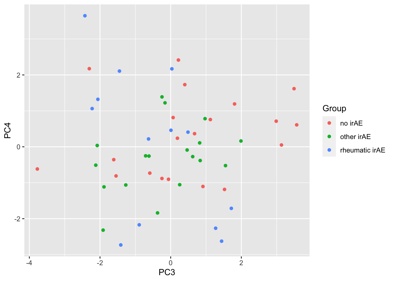

Any PC separate different group?

testTab <- pcTab %>% select(sampleID, PC1:PC20, Group) %>%
    pivot_longer(-c(sampleID, Group)) 
resTab <- group_by(testTab, name) %>% nest() %>%
    mutate(m = map(data, ~aov(lm(value ~ Group,.)))) %>%
    mutate(res = map(m, broom::tidy)) %>%
    unnest(res) %>%
    filter(term == "Group") %>% arrange(p.value)
resTab %>% select(name, p.value) %>% filter(p.value <=0.05)

# A tibble: 2 × 2
# Groups:   name [2]
  name   p.value
  <chr>    <dbl>
1 PC2   0.000295
2 PC1   0.0280

ANOVA

resTab <- subTab %>% group_by(name) %>% nest() %>%
    mutate(m = map(data, ~aov(lm(logVal ~ Group,.)))) %>%
    mutate(res = map(m, broom::tidy)) %>%
    unnest(res) %>%
    filter(term == "Group") %>%
    arrange(p.value) %>%
    select(name, p.value)
resTab.sig <- filter(resTab, p.value < 0.05)
resTab.sig

# A tibble: 11 × 2
# Groups:   name [11]
   name         p.value
   <chr>          <dbl>
 1 IL-33      0.0000484
 2 IL-10      0.000209 
 3 IL-12p70   0.000258 
 4 IL-1beta   0.00821  
 5 Perforin   0.0113   
 6 IFN-alpha2 0.0138   
 7 IFN-gamma  0.0148   
 8 IL-6       0.0276   
 9 IL-17A     0.0296   
10 IL-23      0.0304   
11 GM-CSF     0.0388

Plot

plotTab <- filter(subTab, name %in% resTab.sig$name)
ggplot(plotTab, aes(x=Group, y=logVal)) +
    geom_boxplot() + geom_point() +
    facet_wrap(~name, scales = "free")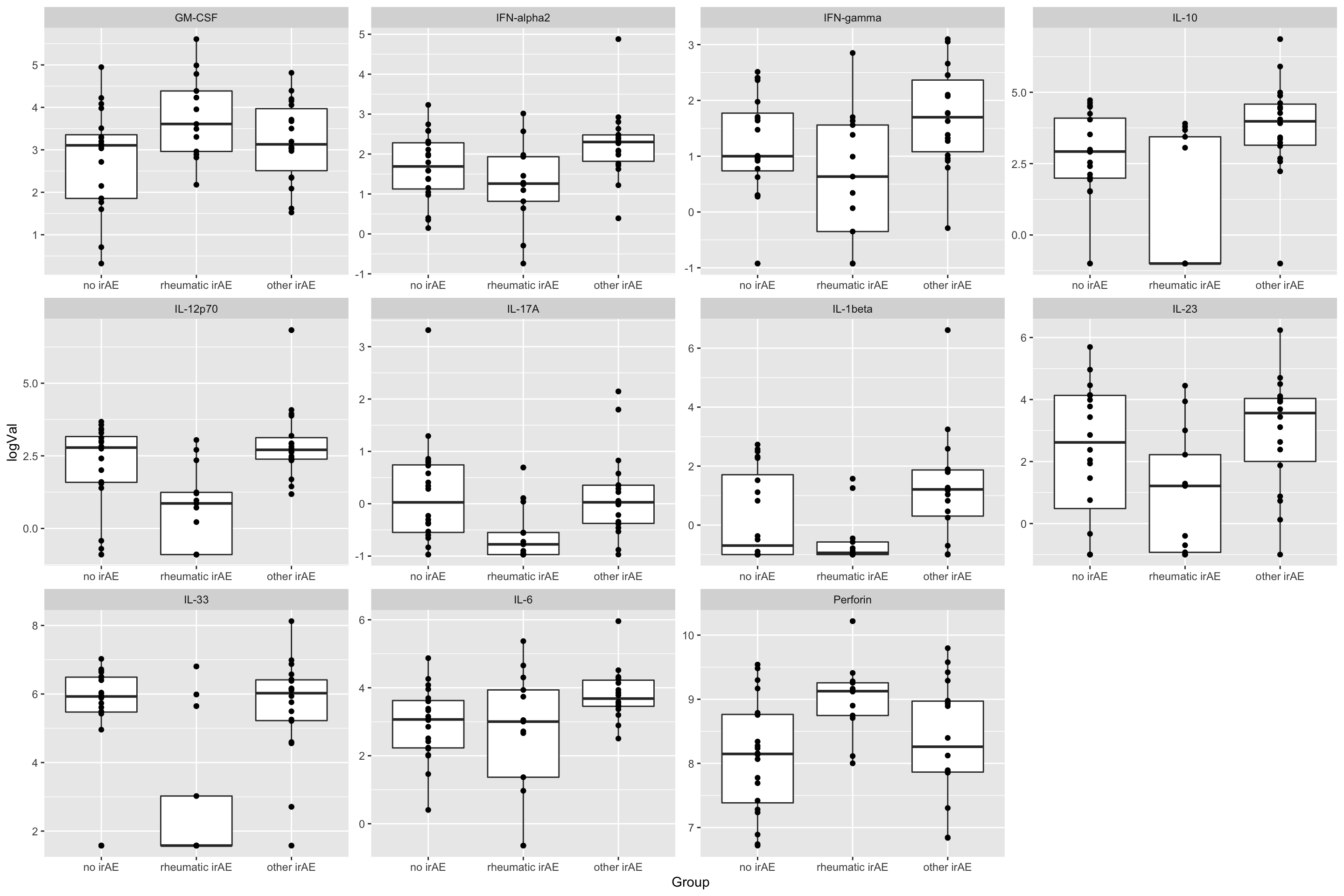

Pair-wise comparison

resPair.followup <- pairwiseT(subTab, "logVal", "Group", "name")
filter(resPair.followup, p.value < 0.05)

# A tibble: 19 × 6
   feature    estimate   p.value group1         group2           p.adj
   <chr>         <dbl>     <dbl> <chr>          <chr>            <dbl>
 1 IL-33         2.67  0.000294  no irAE        rheumatic irAE 0.00764
 2 Perforin     -0.915 0.00242   no irAE        rheumatic irAE 0.0315 
 3 IL-12p70      1.48  0.00612   no irAE        rheumatic irAE 0.0530 
 4 IL-10         1.94  0.00830   no irAE        rheumatic irAE 0.0540 
 5 GM-CSF       -0.992 0.0175    no irAE        rheumatic irAE 0.0822 
 6 IL-17A        0.755 0.0190    no irAE        rheumatic irAE 0.0822 
 7 IL-6         -0.878 0.00581   no irAE        other irAE     0.151  
 8 Granzyme     -2.86  0.0476    no irAE        other irAE     0.345  
 9 IL-12p70     -2.17  0.0000880 rheumatic irAE other irAE     0.00125
10 IL-33        -2.86  0.0000964 rheumatic irAE other irAE     0.00125
11 IL-10        -3.02  0.000224  rheumatic irAE other irAE     0.00194
12 IL-1beta     -1.77  0.00316   rheumatic irAE other irAE     0.0205 
13 IL-23        -2.01  0.00665   rheumatic irAE other irAE     0.0272 
14 IFN-gamma    -1.07  0.00728   rheumatic irAE other irAE     0.0272 
15 IFN-alpha2   -0.997 0.00754   rheumatic irAE other irAE     0.0272 
16 IL-17A       -0.733 0.00837   rheumatic irAE other irAE     0.0272 
17 IL-6         -1.15  0.0259    rheumatic irAE other irAE     0.0749 
18 Perforin      0.642 0.0315    rheumatic irAE other irAE     0.0819 
19 IL-4          2.25  0.0475    rheumatic irAE other irAE     0.112

Use difference between follow_up and baseline

In this analysis, instead of looking at baseline and follow up separately, I created new features by using: follow_up - baseline, which indicates the change over time.

subTab <- filter(cbaTab, assay == "CBA", condition %in% c("Baseline", "Follow_Up")) %>%
    select(name, Group, condition, logVal, patID) %>%
    pivot_wider(names_from = condition, values_from = logVal) %>%
    mutate(diffVal = Follow_Up - Baseline) %>%
    filter(!is.na(diffVal))

PCA

subMat <- subTab %>% select(patID, name, diffVal) %>%
    pivot_wider(names_from = name, values_from = diffVal) %>%
    column_to_rownames("patID") %>% as.matrix()

pcRes <- prcomp(subMat, center = TRUE, scale. = TRUE)
pcTab <- pcRes$x %>% as_tibble(rownames = "patID") %>%
    left_join(patAnno, by = "patID")

ggplot(pcTab, aes(x=PC1, y=PC2, col = Group)) +
    geom_point()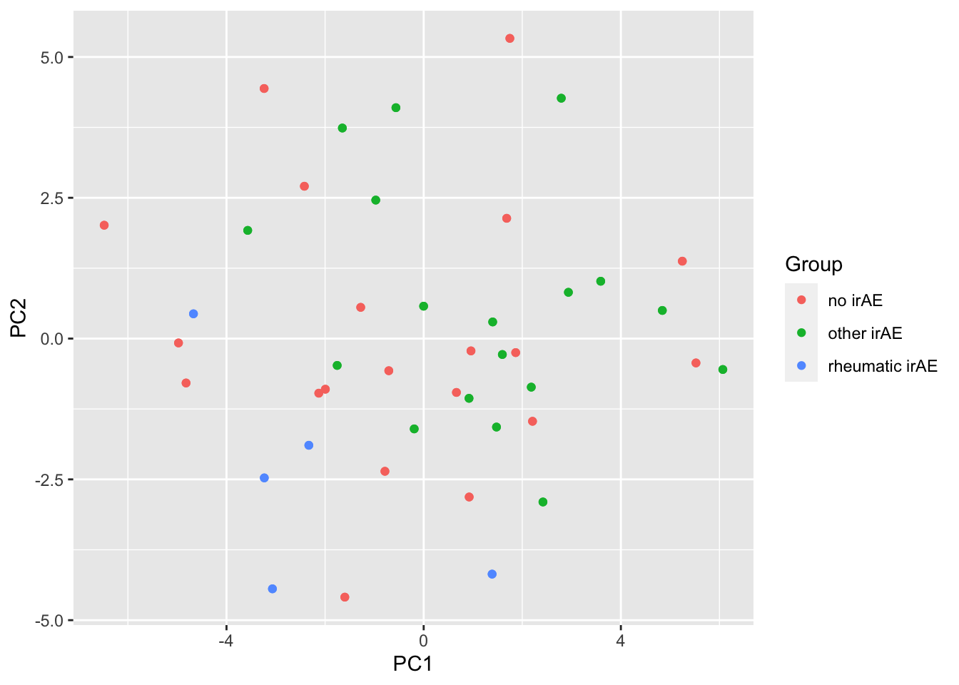

ggplot(pcTab, aes(x=PC3, y=PC4, col = Group)) +
    geom_point()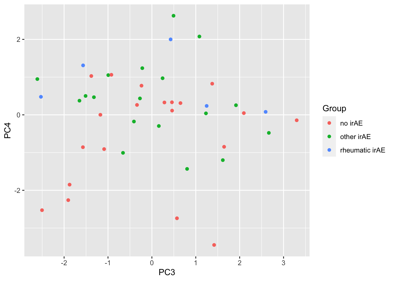

Any PC separate different group?

testTab <- pcTab %>% select(sampleID, PC1:PC20, Group) %>%
    pivot_longer(-c(sampleID, Group)) 
resTab <- group_by(testTab, name) %>% nest() %>%
    mutate(m = map(data, ~aov(lm(value ~ Group,.)))) %>%
    mutate(res = map(m, broom::tidy)) %>%
    unnest(res) %>%
    filter(term == "Group") %>% arrange(p.value)
resTab %>% select(name, p.value) %>% filter(p.value <=0.05)

# A tibble: 6 × 2
# Groups:   name [6]
  name   p.value
  <chr>    <dbl>
1 PC4   0.000585
2 PC2   0.000609
3 PC1   0.000788
4 PC8   0.0145  
5 PC12  0.0194  
6 PC5   0.0426

PC4 versus PC2

ggplot(pcTab, aes(x=PC2, y=PC4, col = Group)) +
    geom_point()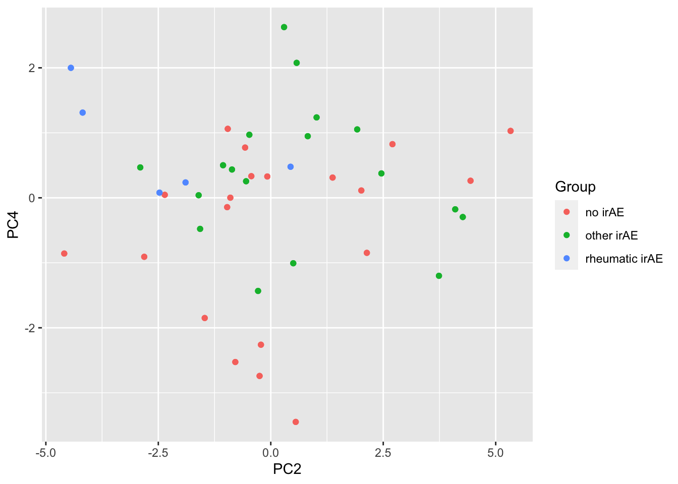

ANOVA

resTab <- subTab %>% group_by(name) %>% nest() %>%
    mutate(m = map(data, ~aov(lm(diffVal ~ Group,.)))) %>%
    mutate(res = map(m, broom::tidy)) %>%
    unnest(res) %>%
    filter(term == "Group") %>%
    arrange(p.value) %>%
    select(name, p.value)
resTab.sig <- filter(resTab, p.value <= 0.05)
resTab.sig

# A tibble: 11 × 2
# Groups:   name [11]
   name       p.value
   <chr>        <dbl>
 1 IL-12p70   0.00215
 2 IL-33      0.00258
 3 IL-23      0.00527
 4 IL-1beta   0.00852
 5 IL-18      0.00857
 6 IFN-alpha2 0.0118 
 7 IL-17A     0.0159 
 8 IL-4       0.0205 
 9 IL-10      0.0265 
10 IFN-gamma  0.0393 
11 TNF-alpha  0.0480

Plot

plotTab <- filter(subTab, name %in% resTab.sig$name)
ggplot(plotTab, aes(x=Group, y=diffVal)) +
    geom_boxplot() + geom_point() +
    facet_wrap(~name, scales = "free")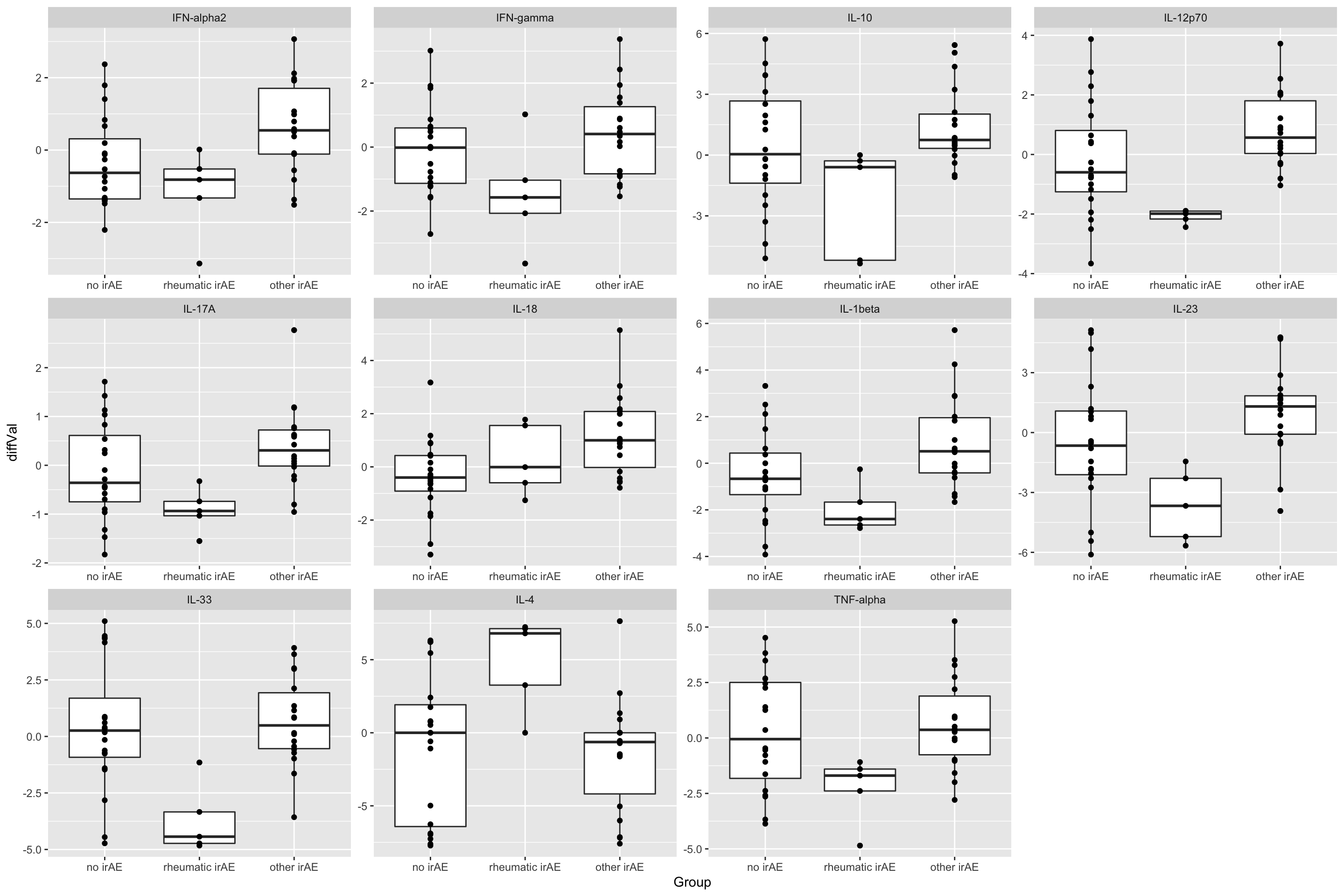

Pair-wise comparison

resPair.diff <- pairwiseT(subTab, "diffVal", "Group", "name")
filter(resPair.diff, p.value <= 0.05)

# A tibble: 19 × 6
   feature    estimate   p.value group1         group2           p.adj
   <chr>         <dbl>     <dbl> <chr>          <chr>            <dbl>
 1 IL-33         4.12  0.00529   no irAE        rheumatic irAE 0.138  
 2 IL-4         -5.83  0.0213    no irAE        rheumatic irAE 0.250  
 3 IL-12p70      1.90  0.0371    no irAE        rheumatic irAE 0.250  
 4 IL-23         3.15  0.0458    no irAE        rheumatic irAE 0.250  
 5 TNF-alpha     2.55  0.0480    no irAE        rheumatic irAE 0.250  
 6 IL-18        -1.56  0.00254   no irAE        other irAE     0.0660 
 7 IFN-alpha2   -0.943 0.0260    no irAE        other irAE     0.289  
 8 IL-1beta     -1.41  0.0334    no irAE        other irAE     0.289  
 9 IL-12p70     -2.89  0.0000528 rheumatic irAE other irAE     0.00137
10 IL-33        -4.36  0.000165  rheumatic irAE other irAE     0.00215
11 IL-23        -4.62  0.000318  rheumatic irAE other irAE     0.00275
12 IL-10        -3.68  0.00247   rheumatic irAE other irAE     0.0142 
13 IL-17A       -1.31  0.00320   rheumatic irAE other irAE     0.0142 
14 IL-4          6.34  0.00327   rheumatic irAE other irAE     0.0142 
15 IL-1beta     -2.85  0.00663   rheumatic irAE other irAE     0.0246 
16 TNF-alpha    -2.95  0.00804   rheumatic irAE other irAE     0.0261 
17 IFN-alpha2   -1.75  0.0118    rheumatic irAE other irAE     0.0341 
18 IFN-gamma    -1.88  0.0172    rheumatic irAE other irAE     0.0447 
19 IL-8         -3.12  0.0395    rheumatic irAE other irAE     0.0934

Summarise the pariwise comparison results using a heatmap

resPair.cba <- bind_rows(
    resPair.baseline %>% mutate(condition = "Baseline"),
    resPair.followup %>% mutate(condition = "Follow_Up"),
    resPair.diff %>% mutate(condition = "Follow_Up - Baseline")
) 
plotTab <- mutate(resPair.cba, 
                  comparison = paste0(group2, " ~ ", group1),
                  logP = -log10(p.value)*sign(estimate),
                  star = case_when(
                      p.value <= 0.01 ~ "**",
                      p.value <= 0.05 ~ "*",
                      TRUE ~ ""
                  ))

ggplot(plotTab, aes(y=feature, x=comparison)) +
    geom_tile(aes(fill = logP)) +
    geom_text(aes(label = star)) +
    facet_wrap(~condition, ncol=3) +
    theme(axis.text.x = element_text(angle = 90, hjust = 1, vjust = 0.5)) +
    scale_fill_gradient2(low = "blue", high="red", midpoint = 0)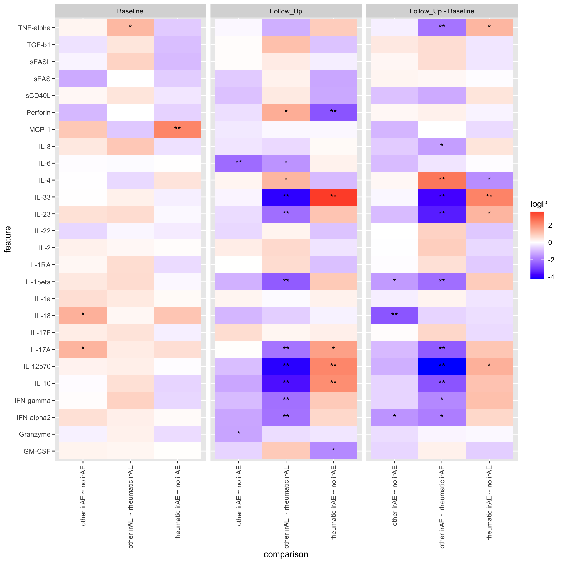

NMR data

nmrTab <- filter(fullTab, assay == "NMR") %>%
    mutate(logVal = value) %>%
    mutate(Group = factor(Group, levels = c("no irAE","rheumatic irAE","other irAE")))

Try vsn transformation (not used, may introduce artefact)

nmrMat <- assays(mae)[["nmr"]]
#vsnFit <- vsn::vsnMatrix(nmrMat, minDataPointsPerStratum = 10)
#nmrMat <- predict(vsnFit, nmrMat)
vsnTab <- nmrMat %>% as_tibble(rownames = "name") %>%
    pivot_longer(-name, names_to = "sampleID", values_to = "logVal")
#nmrTab <- left_join(nmrTab, vsnTab, by =c("sampleID","name"))

Baseline samples

subTab <- filter(nmrTab, condition == "Baseline" )

PCA

subMat <- subTab %>% select(sampleID, name, logVal) %>%
    pivot_wider(names_from = name, values_from = logVal) %>%
    column_to_rownames("sampleID") %>% as.matrix()

pcRes <- prcomp(subMat, center = TRUE, scale. = TRUE)
pcTab <- pcRes$x %>% as_tibble(rownames = "sampleID") %>%
    left_join(patAnno, by = "sampleID")

ggplot(pcTab, aes(x=PC1, y=PC2, col = Group)) +
    geom_point()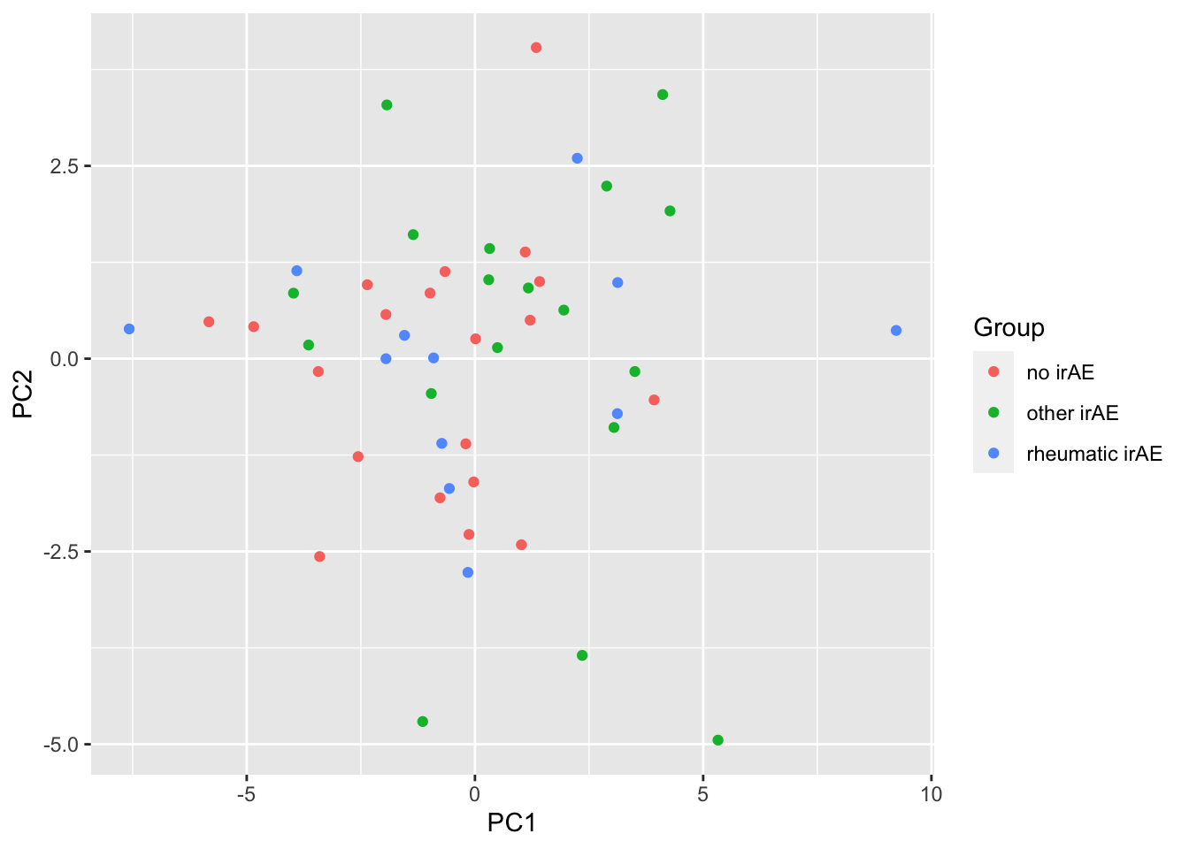

ggplot(pcTab, aes(x=PC3, y=PC4, col = Group)) +
    geom_point()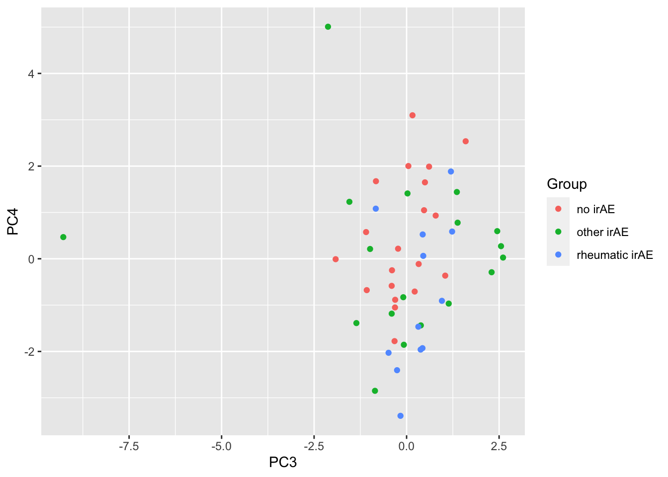

Any PC separate different group?

testTab <- pcTab %>% select(sampleID, PC1:PC20, Group) %>%
    pivot_longer(-c(sampleID, Group)) 
resTab <- group_by(testTab, name) %>% nest() %>%
    mutate(m = map(data, ~aov(lm(value ~ Group,.)))) %>%
    mutate(res = map(m, broom::tidy)) %>%
    unnest(res) %>%
    filter(term == "Group") %>% arrange(p.value)
resTab %>% select(name, p.value) %>% filter(p.value <=0.05)

# A tibble: 2 × 2
# Groups:   name [2]
  name  p.value
  <chr>   <dbl>
1 PC12   0.0132
2 PC11   0.0162

ggplot(pcTab, aes(x=PC11, y=PC12, col = Group)) +
    geom_point()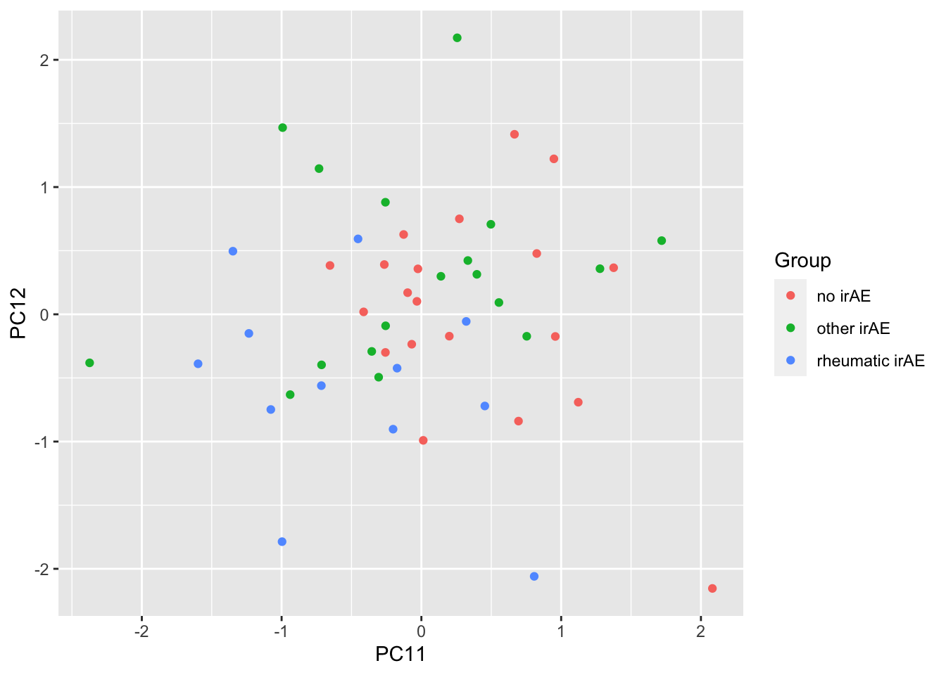

ANOVA

resTab <- subTab %>% group_by(name) %>% nest() %>%
    mutate(m = map(data, ~aov(lm(logVal ~ Group,.)))) %>%
    mutate(res = map(m, broom::tidy)) %>%
    unnest(res) %>%
    filter(term == "Group") %>%
    arrange(p.value) %>%
    select(name, p.value)
resTab.sig <- filter(resTab, p.value < 0.05)
resTab.sig

# A tibble: 1 × 2
# Groups:   name [1]
  name       p.value
  <chr>        <dbl>
1 Histidine 0.000554

Plot

plotTab <- filter(subTab, name %in% resTab.sig$name)
ggplot(plotTab, aes(x=Group, y=logVal)) +
    geom_boxplot() + geom_point() +
    facet_wrap(~name, scales = "free")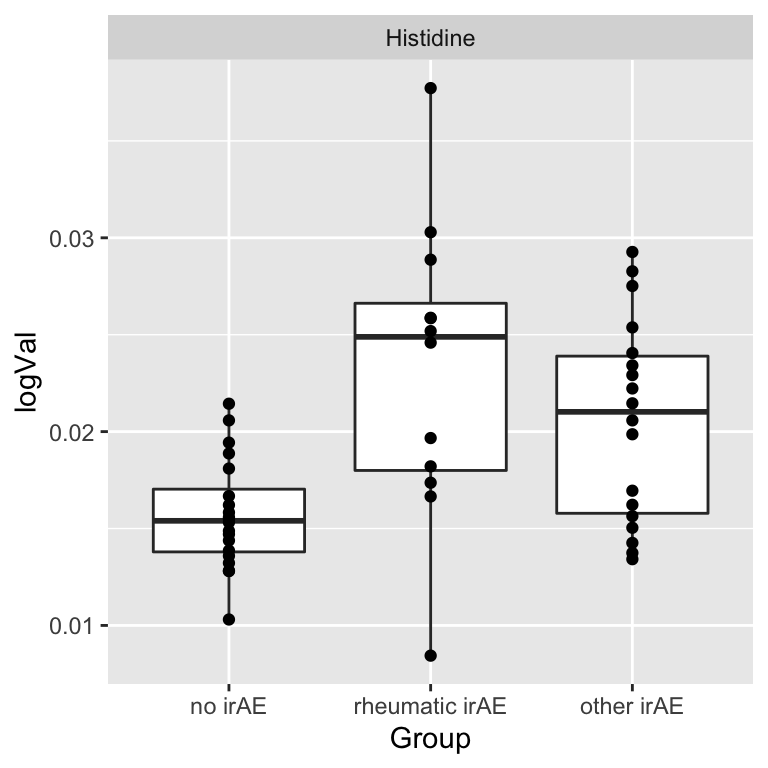

Pair-wise comparison

resPair.baseline <- pairwiseT(subTab, "logVal", "Group", "name")
filter(resPair.baseline, p.value < 0.05)

# A tibble: 6 × 6
  feature    estimate  p.value group1         group2          p.adj
  <chr>         <dbl>    <dbl> <chr>          <chr>           <dbl>
1 Histidine  -0.00752 0.000384 no irAE        rheumatic irAE 0.0127
2 Alanine    -0.0248  0.0379   no irAE        rheumatic irAE 0.603 
3 Histidine  -0.00486 0.000869 no irAE        other irAE     0.0287
4 Asparagine -0.00672 0.0219   no irAE        other irAE     0.362 
5 Leucine    -0.0107  0.0349   no irAE        other irAE     0.384 
6 Succinate  -0.00150 0.0357   rheumatic irAE other irAE     0.857

Follow-up samples

subTab <- filter(nmrTab, condition == "Follow_Up" )

PCA

subMat <- subTab %>% select(sampleID, name, logVal) %>%
    pivot_wider(names_from = name, values_from = logVal) %>%
    column_to_rownames("sampleID") %>% as.matrix()

pcRes <- prcomp(subMat, center = TRUE, scale. = TRUE)
pcTab <- pcRes$x %>% as_tibble(rownames = "sampleID") %>%
    left_join(patAnno, by = "sampleID")

ggplot(pcTab, aes(x=PC1, y=PC2, col = Group)) +
    geom_point()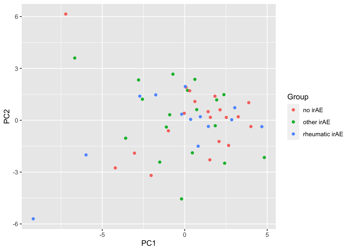

ggplot(pcTab, aes(x=PC3, y=PC4, col = Group)) +
    geom_point()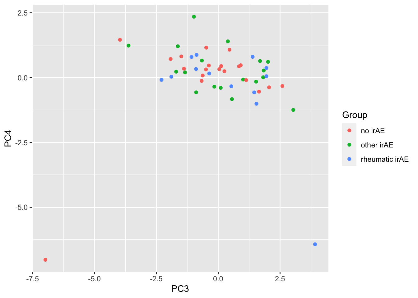

Any PC separate different group?

testTab <- pcTab %>% select(sampleID, PC1:PC20, Group) %>%
    pivot_longer(-c(sampleID, Group)) 
resTab <- group_by(testTab, name) %>% nest() %>%
    mutate(m = map(data, ~aov(lm(value ~ Group,.)))) %>%
    mutate(res = map(m, broom::tidy)) %>%
    unnest(res) %>%
    filter(term == "Group") %>% arrange(p.value)
resTab %>% select(name, p.value) %>% filter(p.value <=0.05)

# A tibble: 2 × 2
# Groups:   name [2]
  name  p.value
  <chr>   <dbl>
1 PC11  0.00789
2 PC13  0.0341

ggplot(pcTab, aes(x=PC11, y=PC13, col = Group)) +
    geom_point()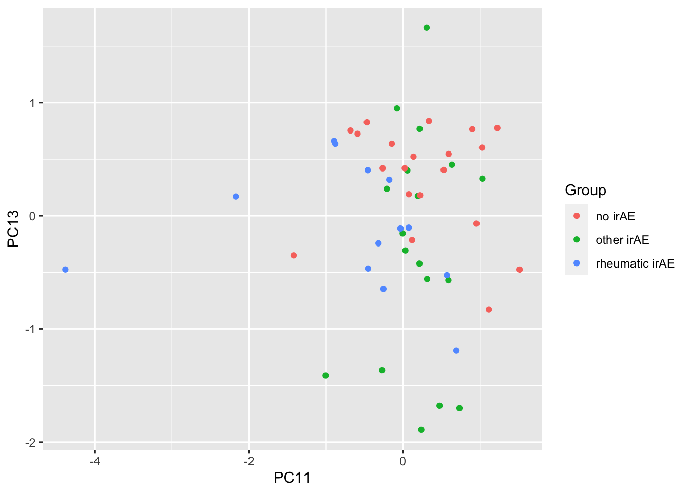

ANOVA

resTab <- subTab %>% group_by(name) %>% nest() %>%
    mutate(m = map(data, ~aov(lm(logVal ~ Group,.)))) %>%
    mutate(res = map(m, broom::tidy)) %>%
    unnest(res) %>%
    filter(term == "Group") %>%
    arrange(p.value) %>%
    select(name, p.value)
resTab.sig <- filter(resTab, p.value < 0.05)
resTab.sig

# A tibble: 2 × 2
# Groups:   name [2]
  name      p.value
  <chr>       <dbl>
1 Histidine  0.0385
2 Glutamine  0.0454

Plot

plotTab <- filter(subTab, name %in% resTab.sig$name)
ggplot(plotTab, aes(x=Group, y=logVal)) +
    geom_boxplot() + geom_point() +
    facet_wrap(~name, scales = "free")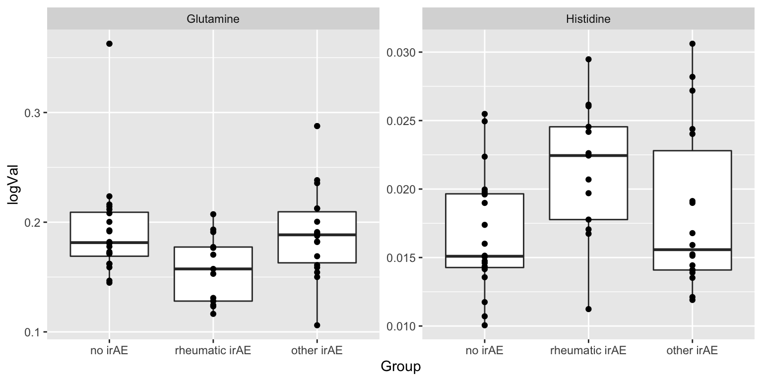

Pair-wise comparison

resPair.followup <- pairwiseT(subTab, "logVal", "Group", "name")
filter(resPair.followup, p.value < 0.05)

# A tibble: 4 × 6
  feature   estimate p.value group1         group2         p.adj
  <chr>        <dbl>   <dbl> <chr>          <chr>          <dbl>
1 Histidine -0.00479 0.00615 no irAE        rheumatic irAE 0.203
2 Glutamine  0.0350  0.0228  no irAE        rheumatic irAE 0.377
3 Acetate   -0.00509 0.0409  no irAE        rheumatic irAE 0.450
4 Glutamine -0.0317  0.0238  rheumatic irAE other irAE     0.786

Use difference between follow_up and baseline

subTab <- filter(nmrTab, condition %in% c("Baseline", "Follow_Up")) %>%
    select(name, Group, condition, logVal, patID) %>%
    pivot_wider(names_from = condition, values_from = logVal) %>%
    mutate(diffVal = Follow_Up - Baseline) %>%
    filter(!is.na(diffVal))

PCA

subMat <- subTab %>% select(patID, name, diffVal) %>%
    pivot_wider(names_from = name, values_from = diffVal) %>%
    column_to_rownames("patID") %>% as.matrix()

pcRes <- prcomp(subMat, center = TRUE, scale. = TRUE)
pcTab <- pcRes$x %>% as_tibble(rownames = "patID") %>%
    left_join(patAnno, by = "patID")

ggplot(pcTab, aes(x=PC1, y=PC2, col = Group)) +
    geom_point()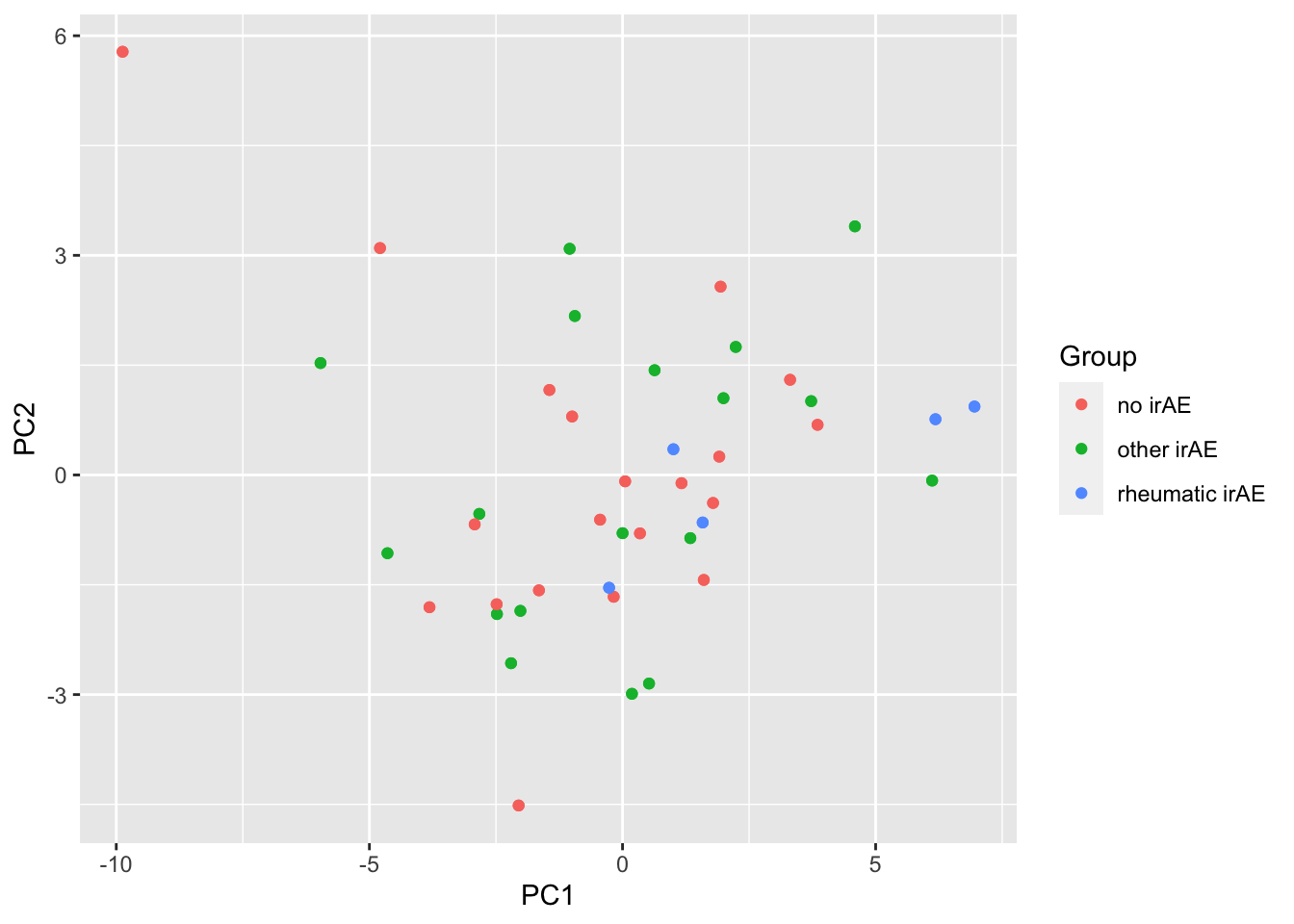

ggplot(pcTab, aes(x=PC3, y=PC4, col = Group)) +
    geom_point()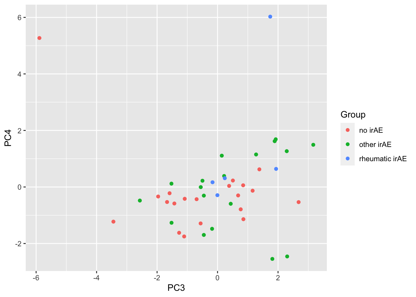

Any PC separate different group?

testTab <- pcTab %>% select(sampleID, PC1:PC20, Group) %>%
    pivot_longer(-c(sampleID, Group)) 
resTab <- group_by(testTab, name) %>% nest() %>%
    mutate(m = map(data, ~aov(lm(value ~ Group,.)))) %>%
    mutate(res = map(m, broom::tidy)) %>%
    unnest(res) %>%
    filter(term == "Group") %>% arrange(p.value)
resTab %>% select(name, p.value) %>% filter(p.value <=0.05)

# A tibble: 9 × 2
# Groups:   name [9]
  name  p.value
  <chr>   <dbl>
1 PC14  0.00146
2 PC1   0.00335
3 PC4   0.0131 
4 PC3   0.0134 
5 PC16  0.0217 
6 PC12  0.0317 
7 PC20  0.0352 
8 PC7   0.0356 
9 PC6   0.0446

ggplot(pcTab, aes(x=PC1, y=PC14, col = Group)) +
    geom_point()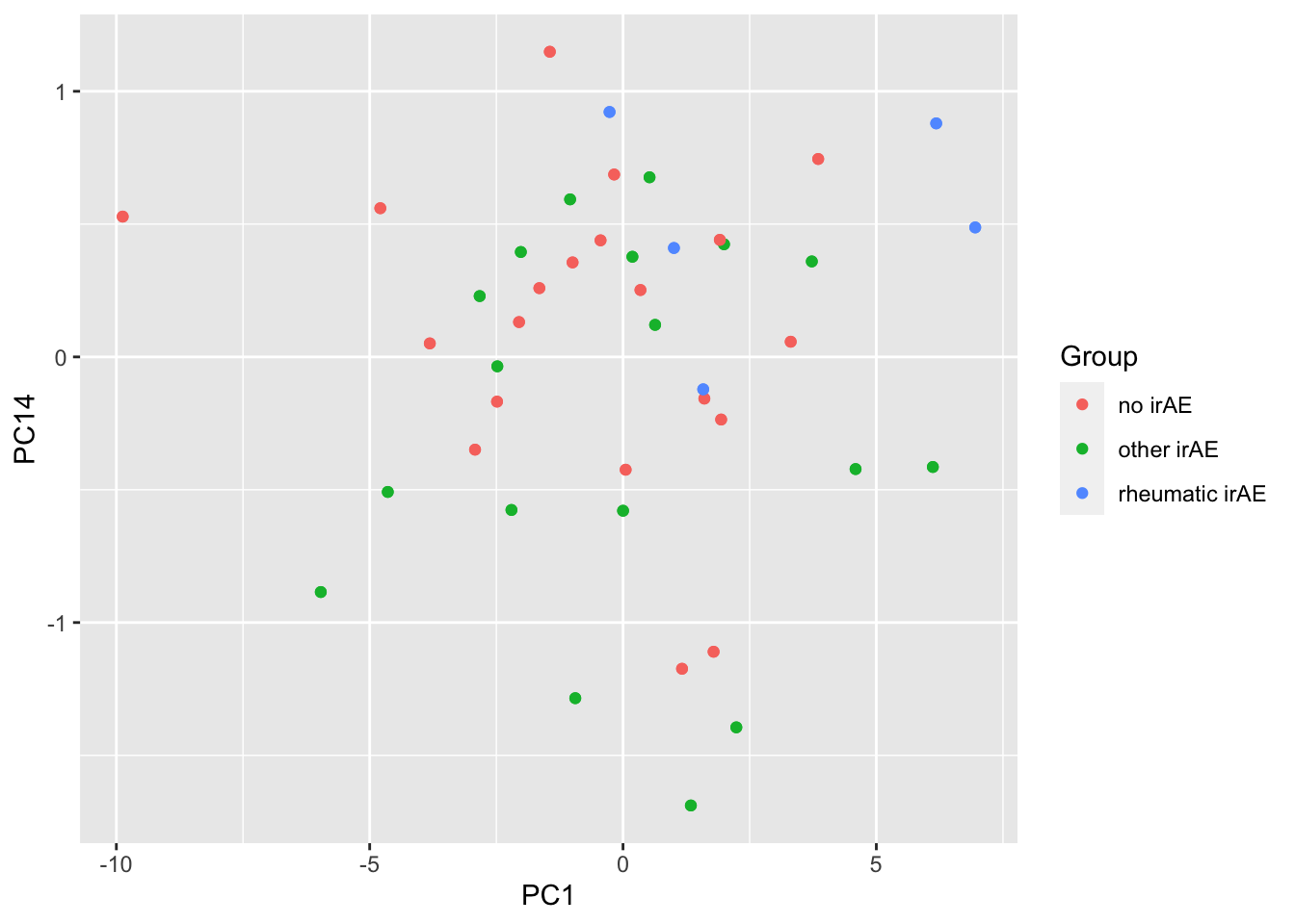

ANOVA

resTab <- subTab %>% group_by(name) %>% nest() %>%
    mutate(m = map(data, ~aov(lm(diffVal ~ Group,.)))) %>%
    mutate(res = map(m, broom::tidy)) %>%
    unnest(res) %>%
    filter(term == "Group") %>%
    arrange(p.value) %>%
    select(name, p.value)
resTab.sig <- filter(resTab, p.value < 0.05)
resTab.sig

# A tibble: 6 × 2
# Groups:   name [6]
  name       p.value
  <chr>        <dbl>
1 Choline     0.0137
2 Alanine     0.0140
3 Leucine     0.0182
4 Valine      0.0238
5 Histidine   0.0277
6 Asparagine  0.0380

Plot

plotTab <- filter(subTab, name %in% resTab.sig$name)
ggplot(plotTab, aes(x=Group, y=diffVal)) +
    geom_boxplot() + geom_point() +
    facet_wrap(~name, scales = "free")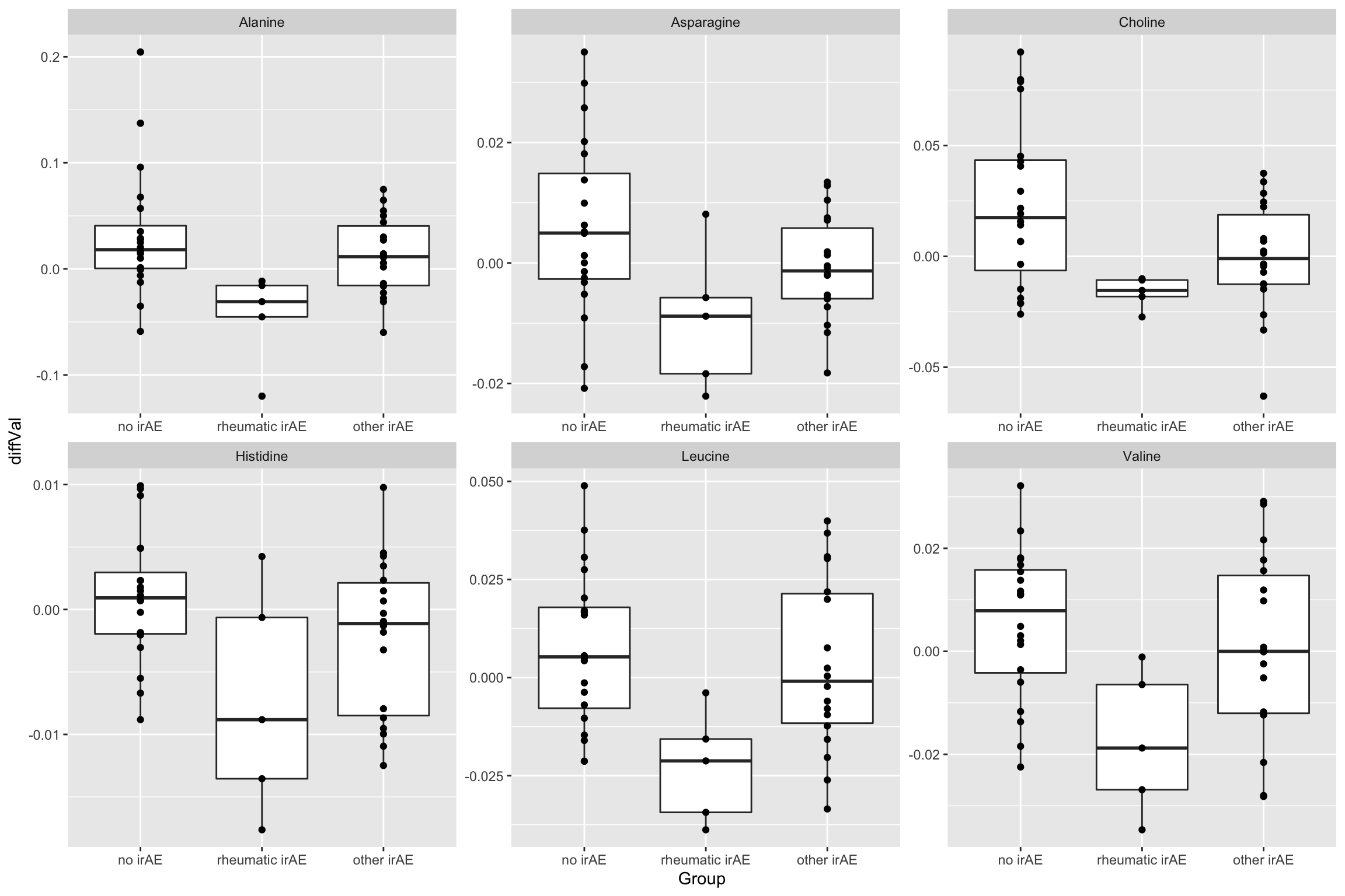

Pair-wise comparison

resPair.diff <- pairwiseT(subTab, "diffVal", "Group", "name")
filter(resPair.diff, p.value < 0.05)

# A tibble: 14 × 6
   feature    estimate p.value group1         group2          p.adj
   <chr>         <dbl>   <dbl> <chr>          <chr>           <dbl>
 1 Leucine     0.0303  0.00408 no irAE        rheumatic irAE 0.0691
 2 Valine      0.0229  0.00419 no irAE        rheumatic irAE 0.0691
 3 Histidine   0.00822 0.0114  no irAE        rheumatic irAE 0.115 
 4 Alanine     0.0761  0.0139  no irAE        rheumatic irAE 0.115 
 5 Choline     0.0395  0.0284  no irAE        rheumatic irAE 0.188 
 6 Proline     0.00988 0.0411  no irAE        rheumatic irAE 0.202 
 7 Asparagine  0.0152  0.0439  no irAE        rheumatic irAE 0.202 
 8 Choline     0.0238  0.0280  no irAE        other irAE     0.796 
 9 Alanine    -0.0569  0.00789 rheumatic irAE other irAE     0.186 
10 Glutamine  -0.0330  0.0113  rheumatic irAE other irAE     0.186 
11 Leucine    -0.0259  0.0231  rheumatic irAE other irAE     0.231 
12 Tyrosine   -0.00631 0.0280  rheumatic irAE other irAE     0.231 
13 Glutamate  -0.0271  0.0447  rheumatic irAE other irAE     0.259 
14 Valine     -0.0183  0.0471  rheumatic irAE other irAE     0.259

Summarise the pariwise comparison results using a heatmap

resPair.cba <- bind_rows(
    resPair.baseline %>% mutate(condition = "Baseline"),
    resPair.followup %>% mutate(condition = "Follow_Up"),
    resPair.diff %>% mutate(condition = "Follow_Up - Baseline")
) 
plotTab <- mutate(resPair.cba, 
                  comparison = paste0(group2, " ~ ", group1),
                  logP = -log10(p.value)*sign(estimate),
                  star = case_when(
                      p.value <= 0.01 ~ "**",
                      p.value <= 0.05 ~ "*",
                      TRUE ~ ""
                  ))

ggplot(plotTab, aes(y=feature, x=comparison)) +
    geom_tile(aes(fill = logP)) +
    geom_text(aes(label = star)) +
    facet_wrap(~condition, ncol=3) +
    theme(axis.text.x = element_text(angle = 90, hjust = 1, vjust = 0.5)) +
    scale_fill_gradient2(low = "blue", high="red", midpoint = 0)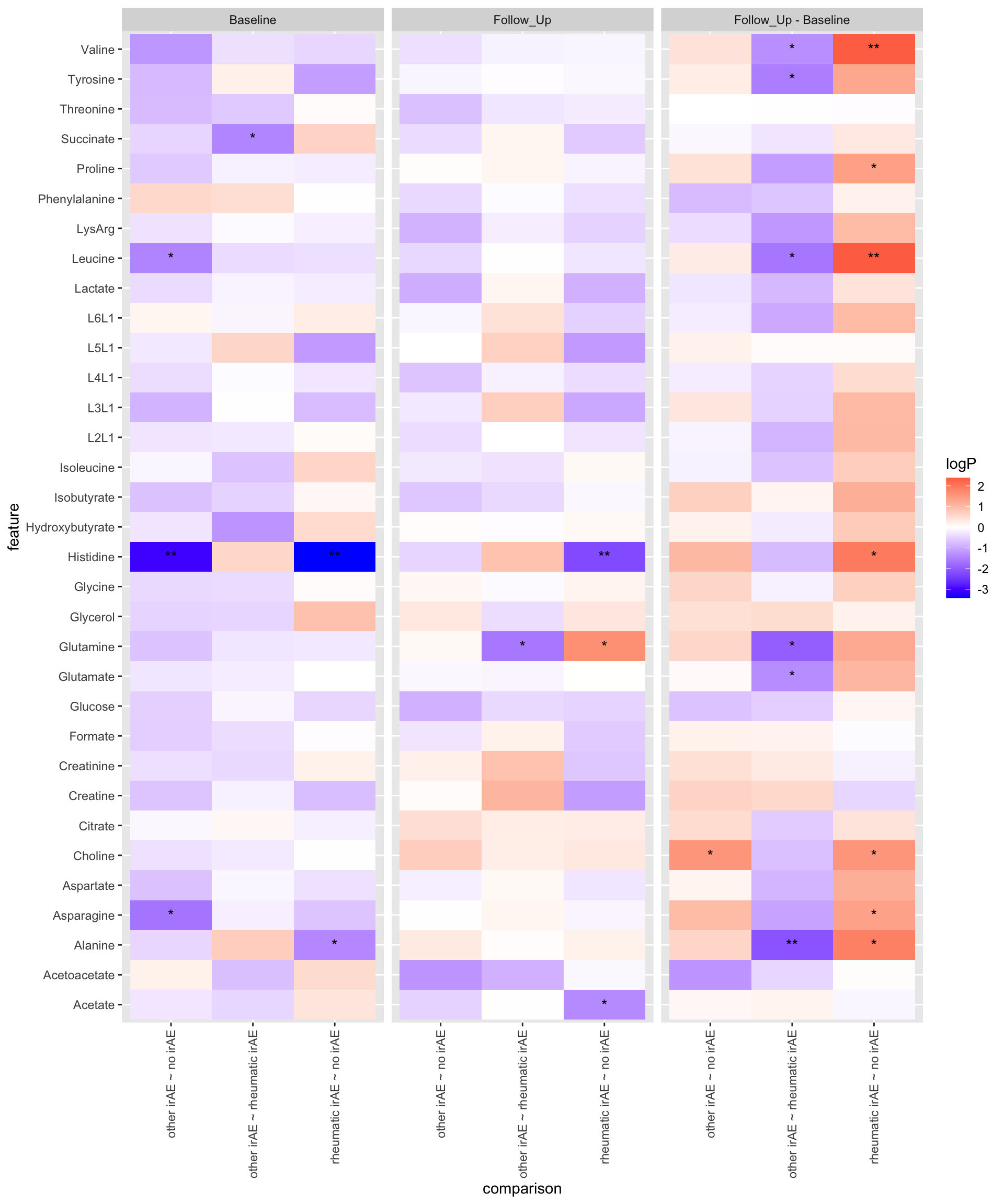

Focuse on cancer patients, combine rheumatic irAE and other irAE into one irAE group

CBA data

cbaTab <- filter(fullTab, assay == "CBA") %>%
    mutate(logVal = glog2(value)) %>%
    mutate(Group2 = ifelse(Group == "no irAE", Group, "irAE")) %>%
    mutate(Group2 = factor(Group2, levels = c("no irAE","irAE")))
patAnno <- mutate(patAnno, Group2 = ifelse(Group == "no irAE", Group, "irAE"))

Baseline samples

subTab <- filter(cbaTab, condition == "Baseline" )

PCA

subMat <- subTab %>% select(sampleID, name, logVal) %>%
    pivot_wider(names_from = name, values_from = logVal) %>%
    column_to_rownames("sampleID") %>% as.matrix()

pcRes <- prcomp(subMat, center = TRUE, scale. = TRUE)
pcTab <- pcRes$x %>% as_tibble(rownames = "sampleID") %>%
    left_join(patAnno, by = "sampleID")

ggplot(pcTab, aes(x=PC1, y=PC2, col = Group2)) +
    geom_point()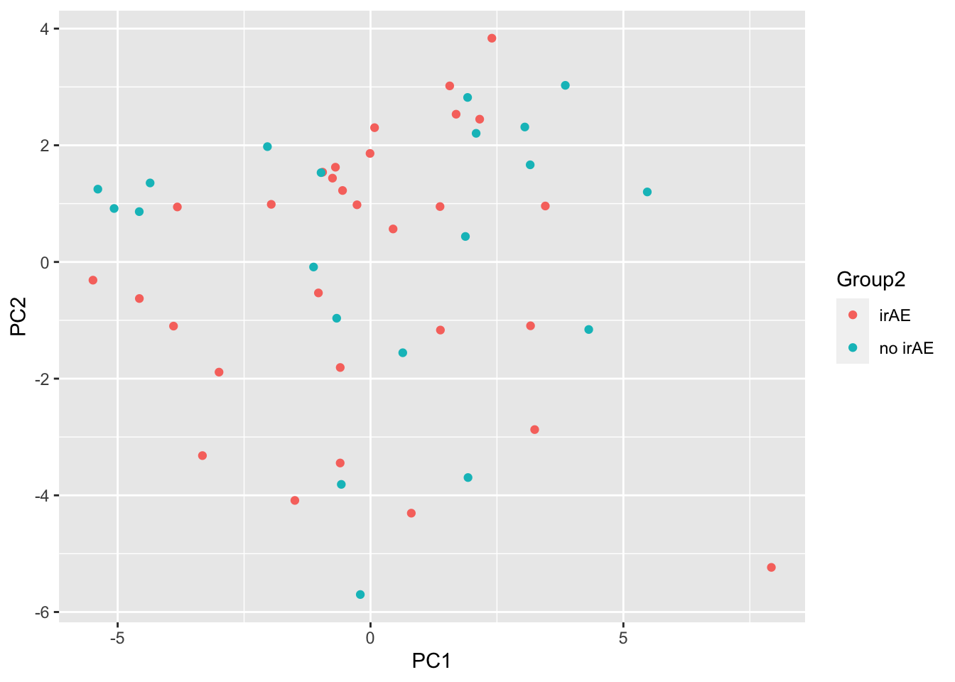

ggplot(pcTab, aes(x=PC3, y=PC4, col = Group2)) +
    geom_point()

Any PC separate different group?

testTab <- pcTab %>% select(sampleID, PC1:PC20, Group2) %>%
    pivot_longer(-c(sampleID, Group2)) 
resTab <- group_by(testTab, name) %>% nest() %>%
    mutate(m = map(data, ~aov(lm(value ~ Group2,.)))) %>%
    mutate(res = map(m, broom::tidy)) %>%
    unnest(res) %>%
    filter(term == "Group2") %>% arrange(p.value)
resTab %>% select(name, p.value) %>% filter(p.value <= 0.05)

# A tibble: 3 × 2
# Groups:   name [3]
  name  p.value
  <chr>   <dbl>
1 PC3   0.00923
2 PC4   0.0141 
3 PC10  0.0423

ggplot(pcTab, aes(x=PC3, y=PC4, col = Group2)) +
    geom_point()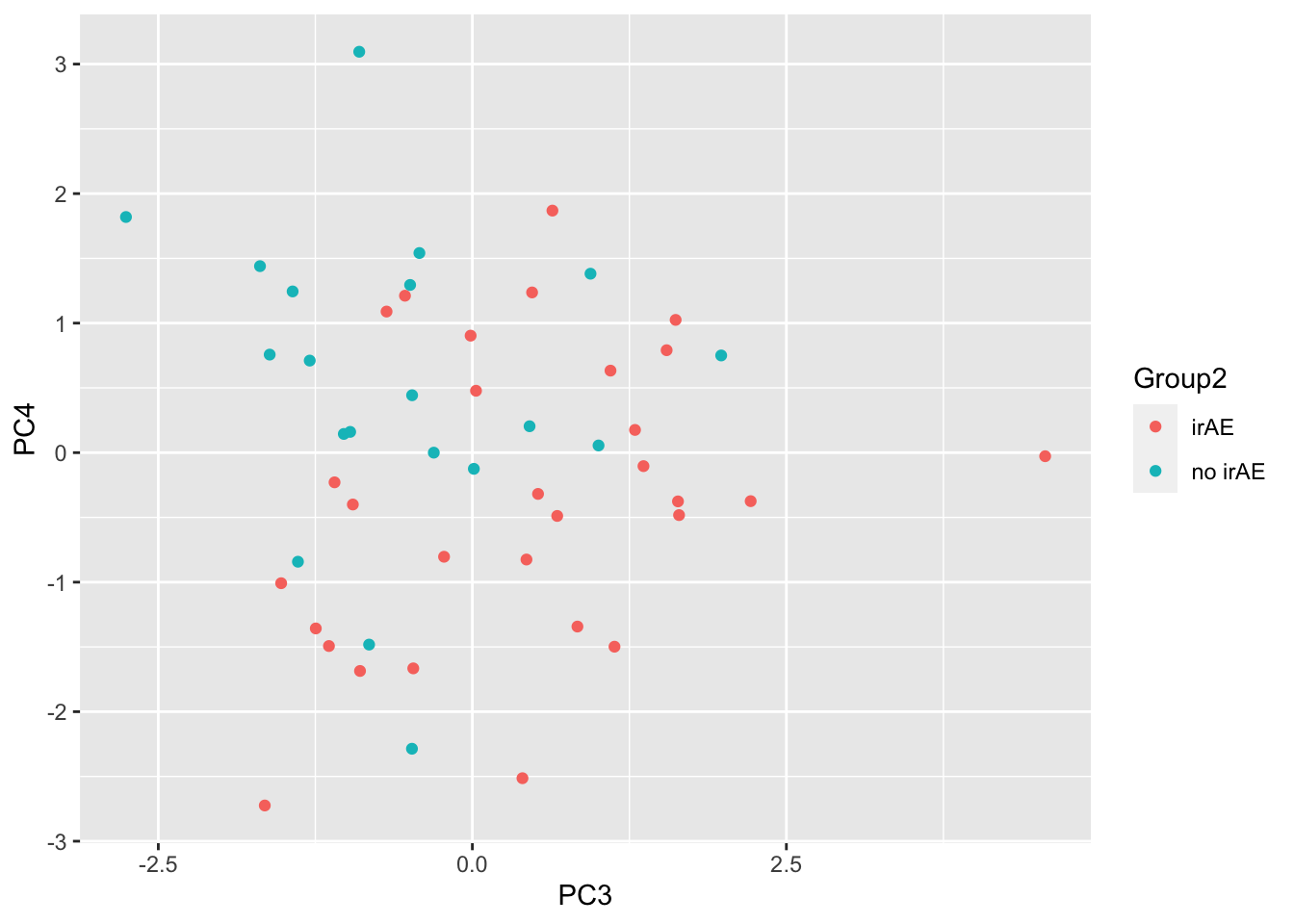

ANOVA

resTab <- subTab %>% group_by(name) %>% nest() %>%
    mutate(m = map(data, ~aov(lm(logVal ~ Group2,.)))) %>%
    mutate(res = map(m, broom::tidy)) %>%
    unnest(res) %>%
    filter(term == "Group2") %>%
    arrange(p.value) %>%
    select(name, p.value)
resTab.sig <- filter(resTab, p.value < 0.05)
resTab.sig

# A tibble: 3 × 2
# Groups:   name [3]
  name   p.value
  <chr>    <dbl>
1 MCP-1   0.0104
2 IL-18   0.0153
3 IL-17A  0.0480

Plot

plotTab <- filter(subTab, name %in% resTab.sig$name)
ggplot(plotTab, aes(x=Group2, y=logVal)) +
    geom_boxplot(outlier.shape = NA) + ggbeeswarm::geom_quasirandom(aes(col=Group)) +
    facet_wrap(~name, scales = "free")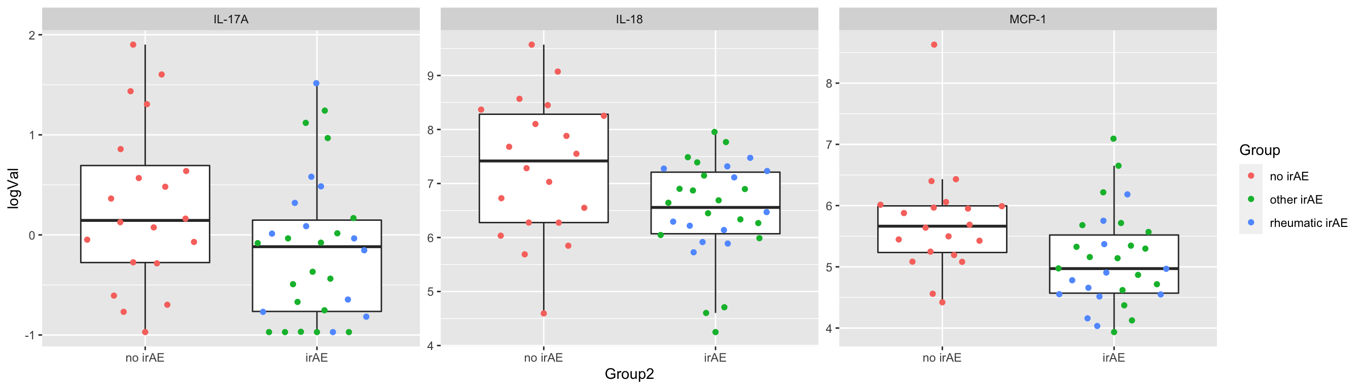

Pair-wise comparison

resPair.baseline <- pairwiseT(subTab, "logVal", "Group2", "name")
#filter(resPair.baseline, p.value < 0.05)

Follow-up samples

subTab <- filter(cbaTab, condition == "Follow_Up" )

PCA

subMat <- subTab %>% select(sampleID, name, logVal) %>%
    pivot_wider(names_from = name, values_from = logVal) %>%
    column_to_rownames("sampleID") %>% as.matrix()

pcRes <- prcomp(subMat, center = TRUE, scale. = TRUE)
pcTab <- pcRes$x %>% as_tibble(rownames = "sampleID") %>%
    left_join(patAnno, by = "sampleID")

ggplot(pcTab, aes(x=PC1, y=PC2, col = Group2)) +
    geom_point()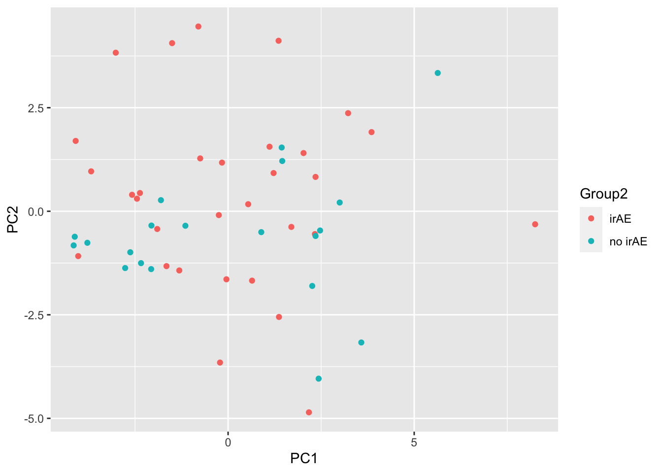

ggplot(pcTab, aes(x=PC3, y=PC4, col = Group2)) +
    geom_point()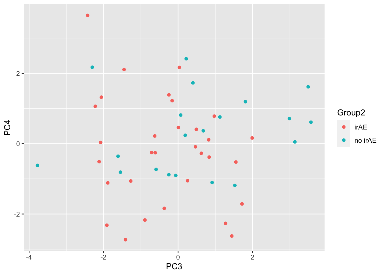

Any PC separate different group?

testTab <- pcTab %>% select(sampleID, PC1:PC20, Group2) %>%
    pivot_longer(-c(sampleID, Group2)) 
resTab <- group_by(testTab, name) %>% nest() %>%
    mutate(m = map(data, ~aov(lm(value ~ Group2,.)))) %>%
    mutate(res = map(m, broom::tidy)) %>%
    unnest(res) %>%
    filter(term == "Group2") %>% arrange(p.value)
resTab %>% select(name, p.value) %>% filter(p.value <=0.05)

# A tibble: 1 × 2
# Groups:   name [1]
  name  p.value
  <chr>   <dbl>
1 PC15   0.0274

ANOVA

resTab <- subTab %>% group_by(name) %>% nest() %>%
    mutate(m = map(data, ~aov(lm(logVal ~ Group2,.)))) %>%
    mutate(res = map(m, broom::tidy)) %>%
    unnest(res) %>%
    filter(term == "Group2") %>%
    arrange(p.value) %>%
    select(name, p.value)
resTab.sig <- filter(resTab, p.value < 0.05)
resTab.sig

# A tibble: 3 × 2
# Groups:   name [3]
  name     p.value
  <chr>      <dbl>
1 Perforin  0.0313
2 sCD40L    0.0343
3 GM-CSF    0.0376

Plot

plotTab <- filter(subTab, name %in% resTab.sig$name)
ggplot(plotTab, aes(x=Group2, y=logVal)) +
    geom_boxplot(outlier.shape = NA) + ggbeeswarm::geom_quasirandom(aes(col=Group)) +
    facet_wrap(~name, scales = "free")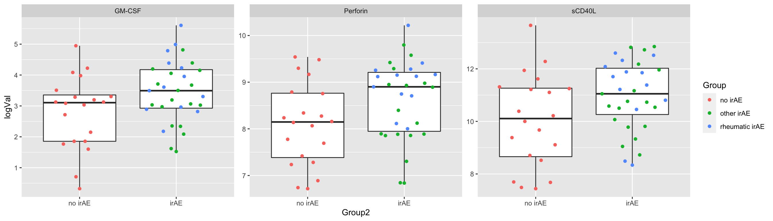

Pair-wise comparison

resPair.followup <- pairwiseT(subTab, "logVal", "Group2", "name")
#filter(resPair.followup, p.value < 0.05)

Difference between follow_up and baseline

subTab <- filter(cbaTab, assay == "CBA", condition %in% c("Baseline", "Follow_Up")) %>%
    select(name, Group, Group2, condition, logVal, patID) %>%
    pivot_wider(names_from = condition, values_from = logVal) %>%
    mutate(diffVal = Follow_Up - Baseline) %>%
    filter(!is.na(diffVal))

PCA

subMat <- subTab %>% select(patID, name, diffVal) %>%
    pivot_wider(names_from = name, values_from = diffVal) %>%
    column_to_rownames("patID") %>% as.matrix()

pcRes <- prcomp(subMat, center = TRUE, scale. = TRUE)
pcTab <- pcRes$x %>% as_tibble(rownames = "patID") %>%
    left_join(patAnno, by = "patID")

ggplot(pcTab, aes(x=PC1, y=PC2, col = Group2)) +
    geom_point()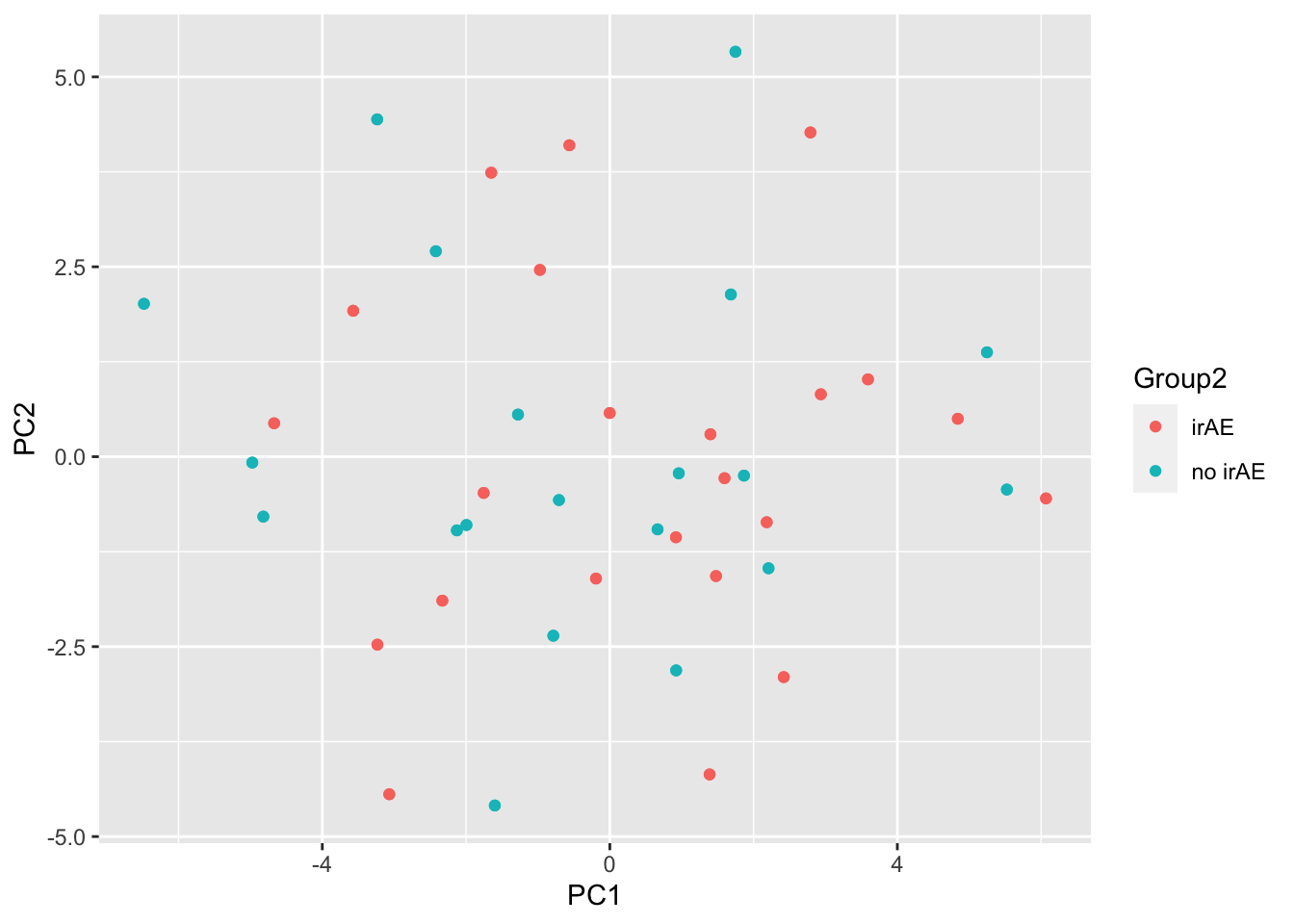

ggplot(pcTab, aes(x=PC3, y=PC4, col = Group2)) +
    geom_point()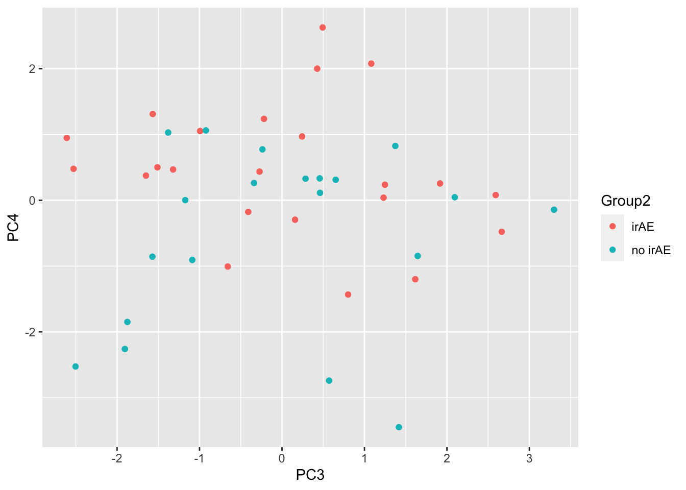

Any PC separate different group?

testTab <- pcTab %>% select(sampleID, PC1:PC20, Group2) %>%
    pivot_longer(-c(sampleID, Group2)) 
resTab <- group_by(testTab, name) %>% nest() %>%
    mutate(m = map(data, ~aov(lm(value ~ Group2,.)))) %>%
    mutate(res = map(m, broom::tidy)) %>%
    unnest(res) %>%
    filter(term == "Group2") %>% arrange(p.value)
resTab %>% select(name, p.value) %>% filter(p.value <=0.05)

# A tibble: 2 × 2
# Groups:   name [2]
  name   p.value
  <chr>    <dbl>
1 PC4   0.000210
2 PC20  0.0448

ggplot(pcTab, aes(x=PC20, y=PC4, col = Group2)) +
    geom_point()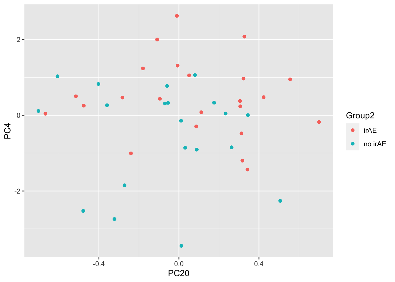

ANOVA

resTab <- subTab %>% group_by(name) %>% nest() %>%
    mutate(m = map(data, ~aov(lm(diffVal ~ Group2,.)))) %>%
    mutate(res = map(m, broom::tidy)) %>%
    unnest(res) %>%
    filter(term == "Group2") %>%
    arrange(p.value) %>%
    select(name, p.value)
resTab.sig <- filter(resTab, p.value < 0.05)
resTab.sig

# A tibble: 1 × 2
# Groups:   name [1]
  name  p.value
  <chr>   <dbl>
1 IL-18 0.00415

Plot

plotTab <- filter(subTab, name %in% resTab.sig$name)
ggplot(plotTab, aes(x=Group2, y=diffVal)) +
    geom_boxplot(outlier.shape = NA) + ggbeeswarm::geom_quasirandom(aes(col=Group)) +
    facet_wrap(~name, scales = "free")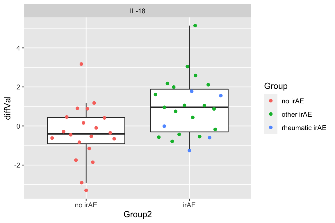

Pair-wise comparison

resPair.diff <- pairwiseT(subTab, "diffVal", "Group2", "name")
#filter(resPair.diff, p.value < 0.05)

Summarise the pariwise comparison results using a heatmap

resPair.cba <- bind_rows(
    resPair.baseline %>% mutate(condition = "Baseline"),
    resPair.followup %>% mutate(condition = "Follow_Up"),
    resPair.diff %>% mutate(condition = "Follow_Up - Baseline")
) 
plotTab <- mutate(resPair.cba, 
                  comparison = paste0(group2, " ~ ", group1),
                  logP = -log10(p.value)*sign(estimate),
                  star = case_when(
                      p.value <= 0.01 ~ "**",
                      p.value <= 0.05 ~ "*",
                      TRUE ~ ""
                  ))

ggplot(plotTab, aes(y=feature, x=comparison)) +
    geom_tile(aes(fill = logP)) +
    geom_text(aes(label = star)) +
    facet_wrap(~condition, ncol=3) +
    theme(axis.text.x = element_text(angle = 90, hjust = 1, vjust = 0.5)) +
    scale_fill_gradient2(low = "blue", high="red")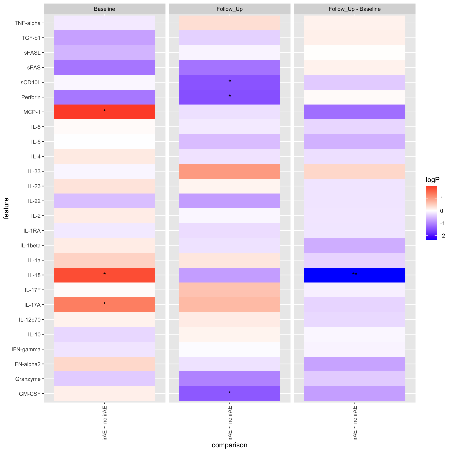

NMR data

nmrTab <- filter(fullTab, assay == "NMR") %>%
    mutate(logVal = value) %>%
    mutate(Group2 = ifelse(Group == "no irAE", Group, "irAE")) %>%
    mutate(Group2 = factor(Group2, levels = c("no irAE","irAE")))
patAnno <- mutate(patAnno, Group2 = ifelse(Group == "no irAE", Group, "irAE"))

Try vsn transformation (not used, may introduce artefact)

nmrMat <- assays(mae)[["nmr"]]
#vsnFit <- vsn::vsnMatrix(nmrMat, minDataPointsPerStratum = 10)
#nmrMat <- predict(vsnFit, nmrMat)
vsnTab <- nmrMat %>% as_tibble(rownames = "name") %>%
    pivot_longer(-name, names_to = "sampleID", values_to = "logVal")
#nmrTab <- left_join(nmrTab, vsnTab, by =c("sampleID","name"))

Baseline samples

subTab <- filter(nmrTab, condition == "Baseline" )

PCA

subMat <- subTab %>% select(sampleID, name, logVal) %>%
    pivot_wider(names_from = name, values_from = logVal) %>%
    column_to_rownames("sampleID") %>% as.matrix()

pcRes <- prcomp(subMat, center = TRUE, scale. = TRUE)
pcTab <- pcRes$x %>% as_tibble(rownames = "sampleID") %>%
    left_join(patAnno, by = "sampleID")

ggplot(pcTab, aes(x=PC1, y=PC2, col = Group2)) +
    geom_point()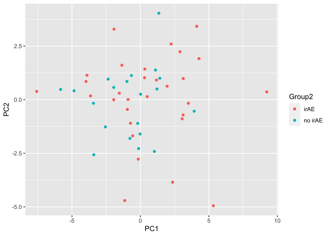

ggplot(pcTab, aes(x=PC3, y=PC4, col = Group2)) +
    geom_point()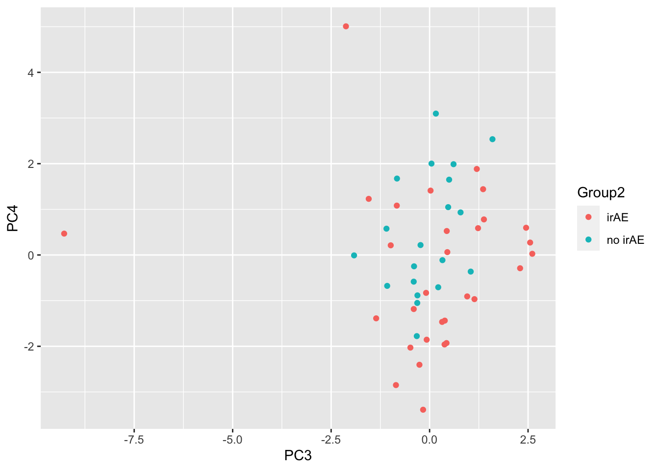

Any PC separate different group?

testTab <- pcTab %>% select(sampleID, PC1:PC20, Group2) %>%
    pivot_longer(-c(sampleID, Group2)) 
resTab <- group_by(testTab, name) %>% nest() %>%
    mutate(m = map(data, ~aov(lm(value ~ Group2,.)))) %>%
    mutate(res = map(m, broom::tidy)) %>%
    unnest(res) %>%
    filter(term == "Group2") %>% arrange(p.value)
resTab %>% select(name, p.value) %>% filter(p.value <=0.05)

# A tibble: 3 × 2
# Groups:   name [3]
  name  p.value
  <chr>   <dbl>
1 PC11   0.0143
2 PC15   0.0166
3 PC13   0.0475

ggplot(pcTab, aes(x=PC11, y=PC15, col = Group2)) +
    geom_point()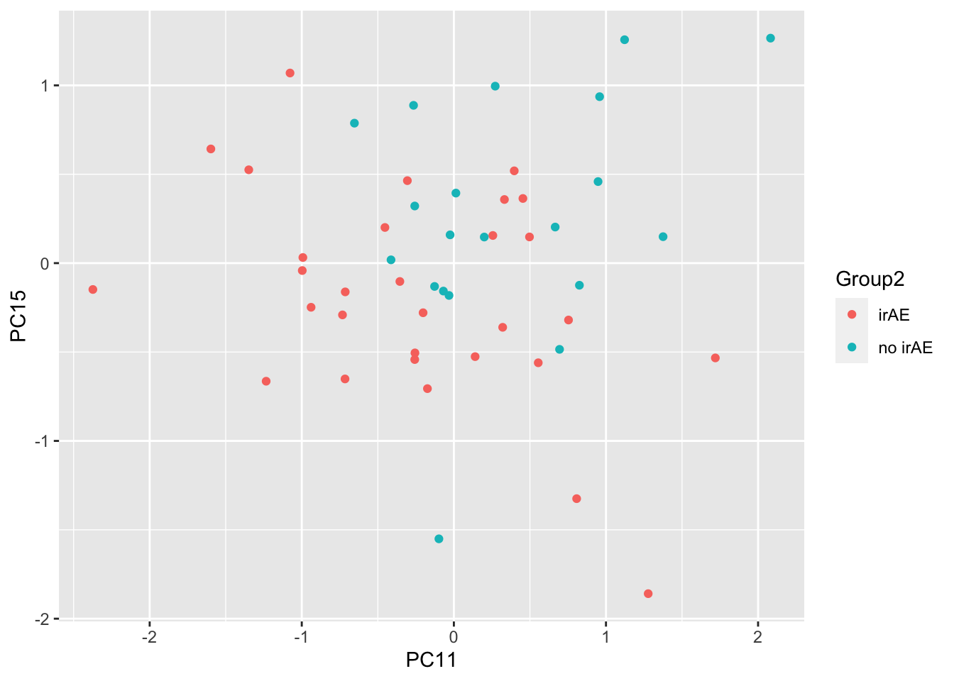

ANOVA

resTab <- subTab %>% group_by(name) %>% nest() %>%
    mutate(m = map(data, ~aov(lm(logVal ~ Group2,.)))) %>%
    mutate(res = map(m, broom::tidy)) %>%
    unnest(res) %>%
    filter(term == "Group2") %>%
    arrange(p.value) %>%
    select(name, p.value)
resTab.sig <- filter(resTab, p.value < 0.05)
resTab.sig

# A tibble: 2 × 2
# Groups:   name [2]
  name        p.value
  <chr>         <dbl>
1 Histidine  0.000269
2 Asparagine 0.0379

Plot

plotTab <- filter(subTab, name %in% resTab.sig$name)
ggplot(plotTab, aes(x=Group2, y=logVal)) +
    geom_boxplot(outlier.shape = NA) + ggbeeswarm::geom_quasirandom(aes(col=Group)) +
    facet_wrap(~name, scales = "free")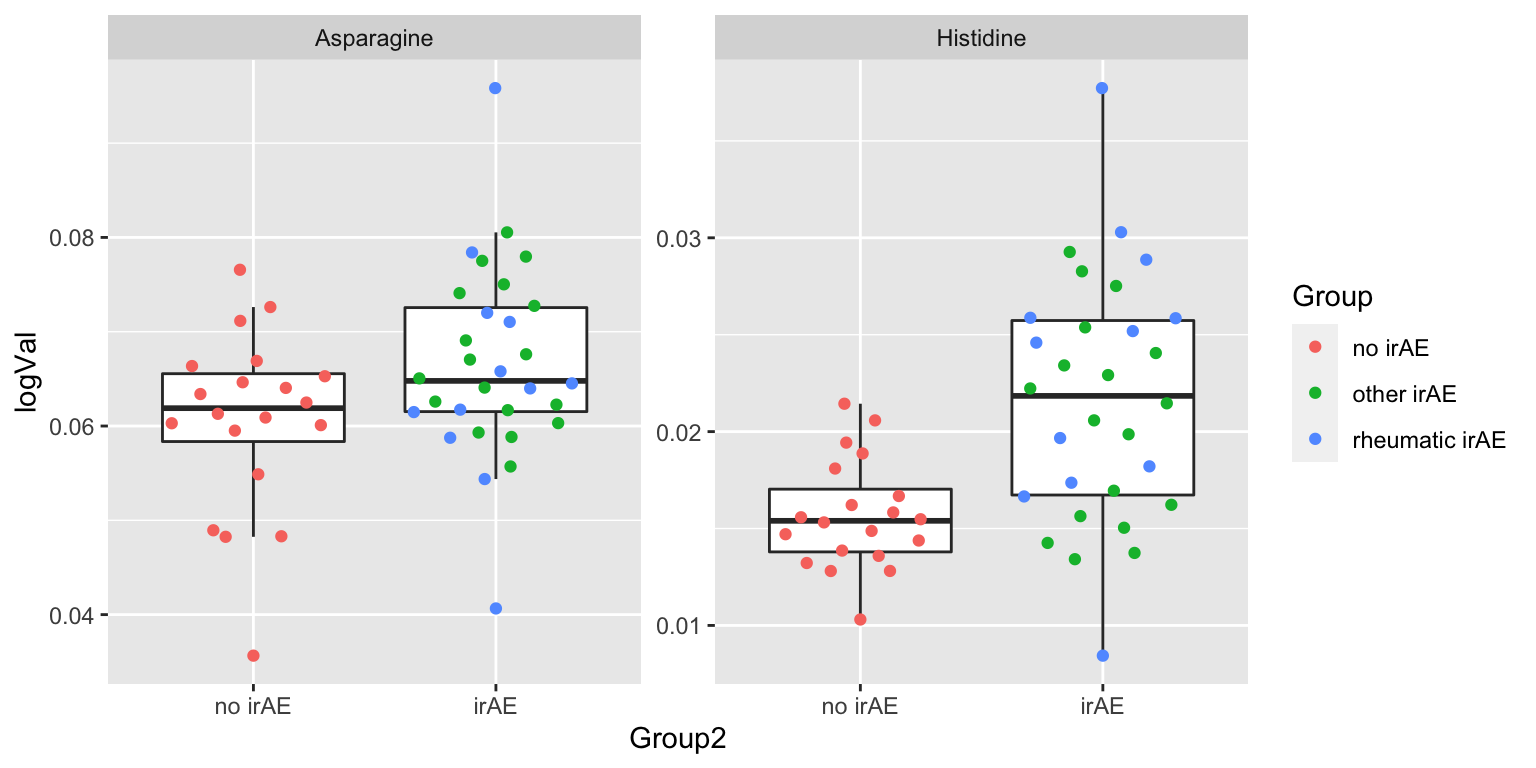

Pair-wise comparison

resPair.baseline <- pairwiseT(subTab, "logVal", "Group2", "name")
#filter(resPair.baseline, p.value < 0.05)

Follow-up samples

subTab <- filter(nmrTab, condition == "Follow_Up" )

PCA

subMat <- subTab %>% select(sampleID, name, logVal) %>%
    pivot_wider(names_from = name, values_from = logVal) %>%
    column_to_rownames("sampleID") %>% as.matrix()

pcRes <- prcomp(subMat, center = TRUE, scale. = TRUE)
pcTab <- pcRes$x %>% as_tibble(rownames = "sampleID") %>%
    left_join(patAnno, by = "sampleID")

ggplot(pcTab, aes(x=PC1, y=PC2, col = Group2)) +
    geom_point()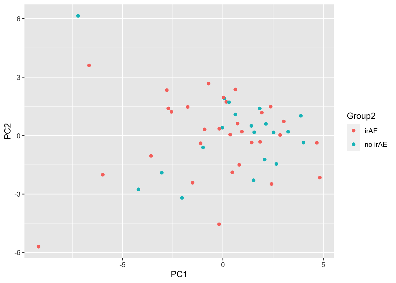

ggplot(pcTab, aes(x=PC3, y=PC4, col = Group2)) +
    geom_point()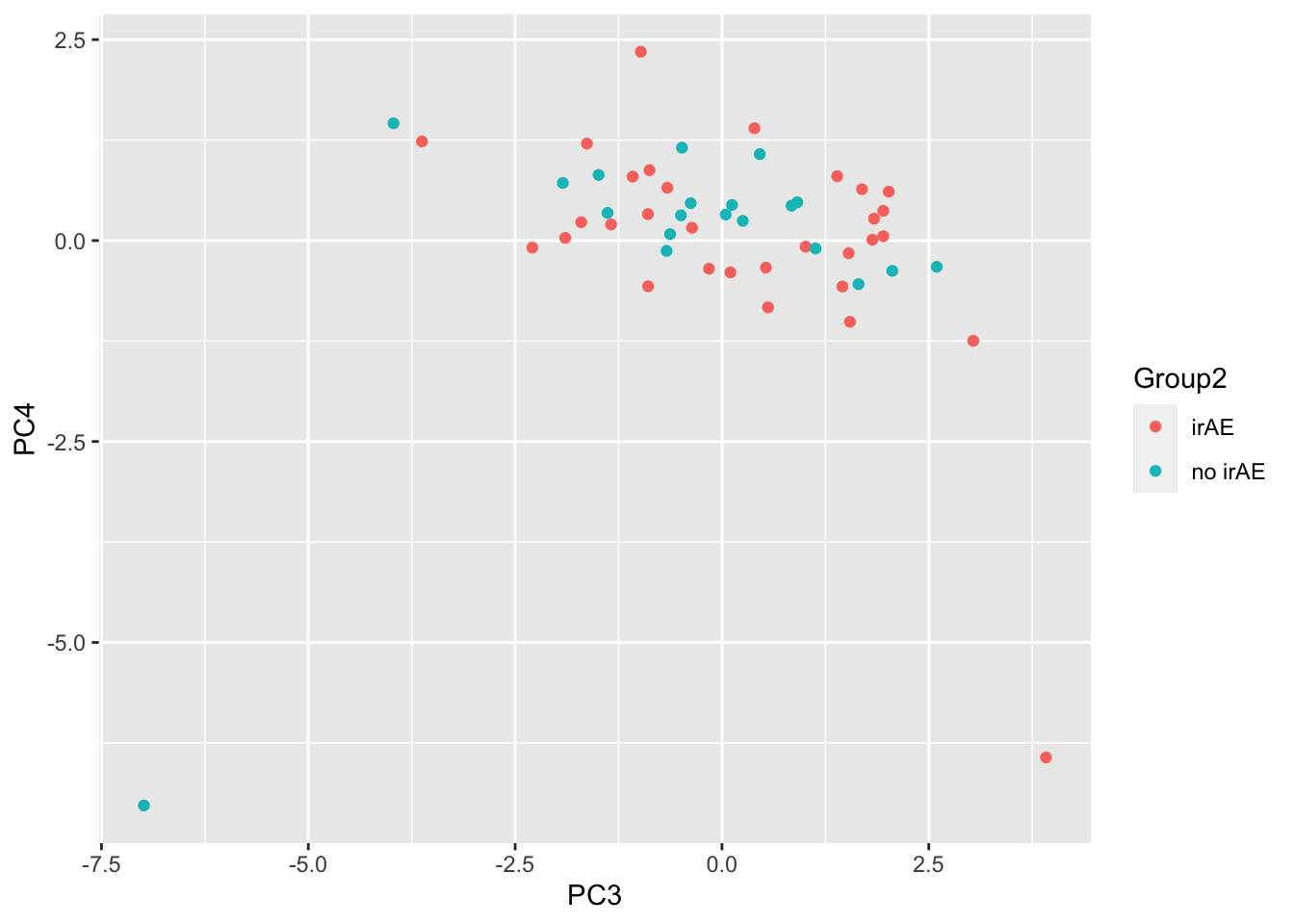

Any PC separate different group?

testTab <- pcTab %>% select(sampleID, PC1:PC20, Group2) %>%
    pivot_longer(-c(sampleID, Group2)) 
resTab <- group_by(testTab, name) %>% nest() %>%
    mutate(m = map(data, ~aov(lm(value ~ Group2,.)))) %>%
    mutate(res = map(m, broom::tidy)) %>%
    unnest(res) %>%
    filter(term == "Group2") %>% arrange(p.value)
resTab %>% select(name, p.value) %>% filter(p.value <=0.05)

# A tibble: 2 × 2
# Groups:   name [2]
  name  p.value
  <chr>   <dbl>
1 PC13   0.0111
2 PC16   0.0454

ggplot(pcTab, aes(x=PC13, y=PC16, col = Group2)) +
    geom_point()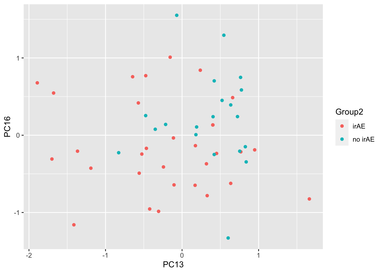

ANOVA

resTab <- subTab %>% group_by(name) %>% nest() %>%
    mutate(m = map(data, ~aov(lm(logVal ~ Group2,.)))) %>%
    mutate(res = map(m, broom::tidy)) %>%
    unnest(res) %>%
    filter(term == "Group2") %>%
    arrange(p.value) %>%
    select(name, p.value)
resTab.sig <- filter(resTab, p.value < 0.1)
resTab.sig

# A tibble: 2 × 2
# Groups:   name [2]
  name      p.value
  <chr>       <dbl>
1 Histidine  0.0513
2 Lactate    0.0827

Plot

plotTab <- filter(subTab, name %in% resTab.sig$name)
ggplot(plotTab, aes(x=Group2, y=logVal)) +
    geom_boxplot(outlier.shape = NA) + ggbeeswarm::geom_quasirandom(aes(col=Group)) +
    facet_wrap(~name, scales = "free")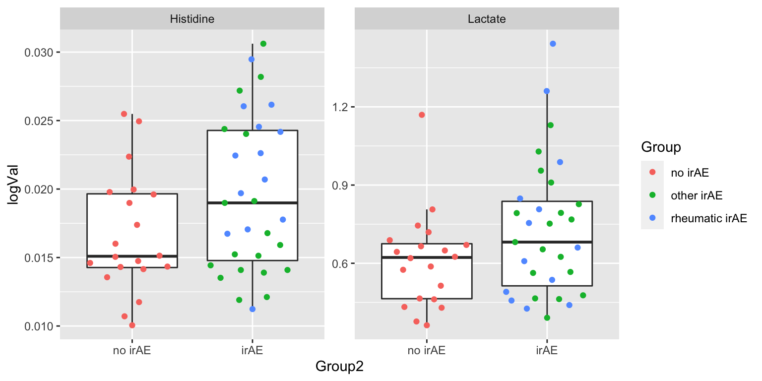

Pair-wise comparison

resPair.followup <- pairwiseT(subTab, "logVal", "Group2", "name")

Use difference between follow_up and baseline

subTab <- filter(nmrTab, condition %in% c("Baseline", "Follow_Up")) %>%
    select(name, Group, condition, Group2,logVal, patID) %>%
    pivot_wider(names_from = condition, values_from = logVal) %>%
    mutate(diffVal = Follow_Up - Baseline) %>%
    filter(!is.na(diffVal))

PCA

subMat <- subTab %>% select(patID, name, diffVal) %>%
    pivot_wider(names_from = name, values_from = diffVal) %>%
    column_to_rownames("patID") %>% as.matrix()

pcRes <- prcomp(subMat, center = TRUE, scale. = TRUE)
pcTab <- pcRes$x %>% as_tibble(rownames = "patID") %>%
    left_join(patAnno, by = "patID")

ggplot(pcTab, aes(x=PC1, y=PC2, col = Group2)) +
    geom_point()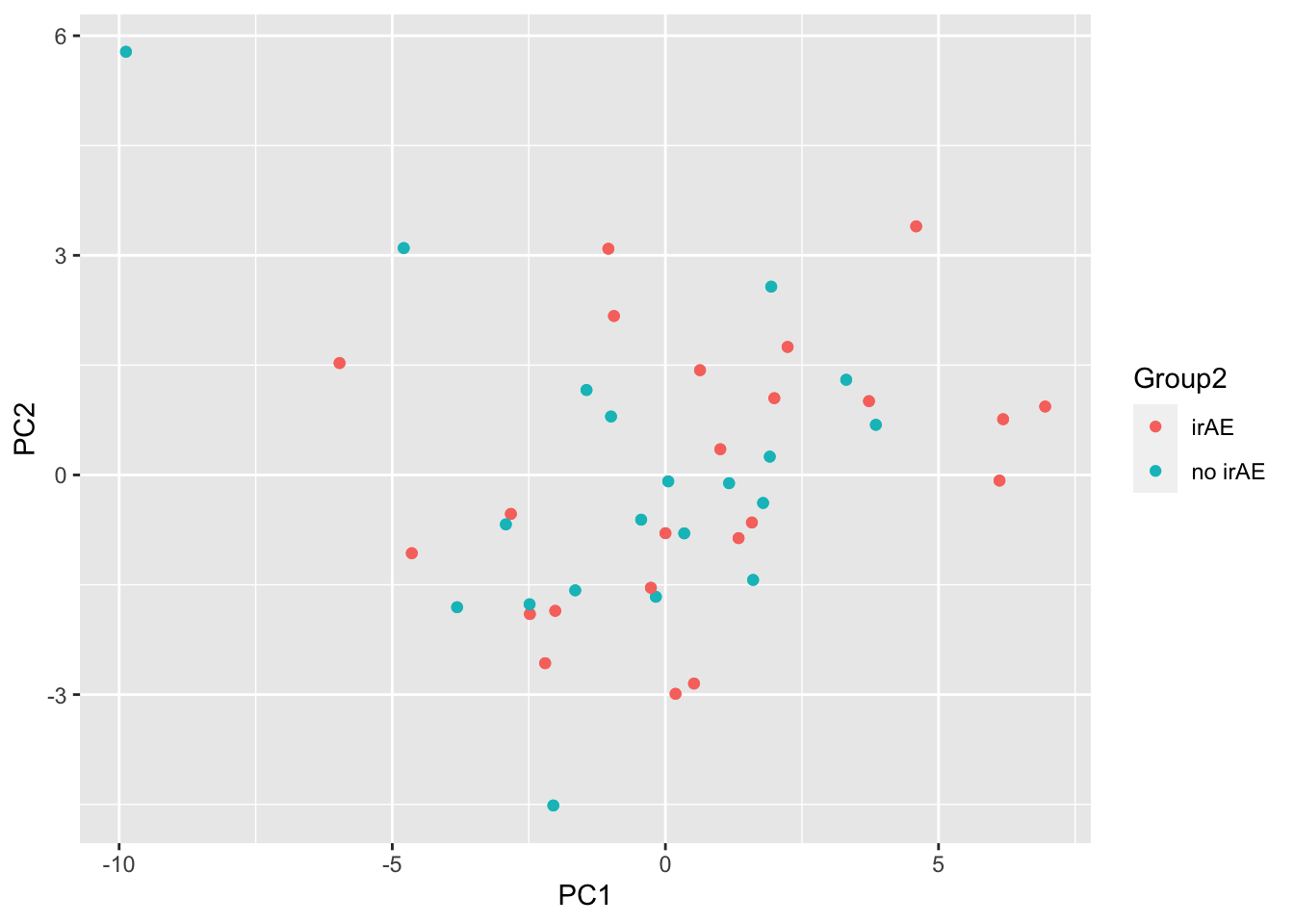

ggplot(pcTab, aes(x=PC3, y=PC4, col = Group2)) +
    geom_point()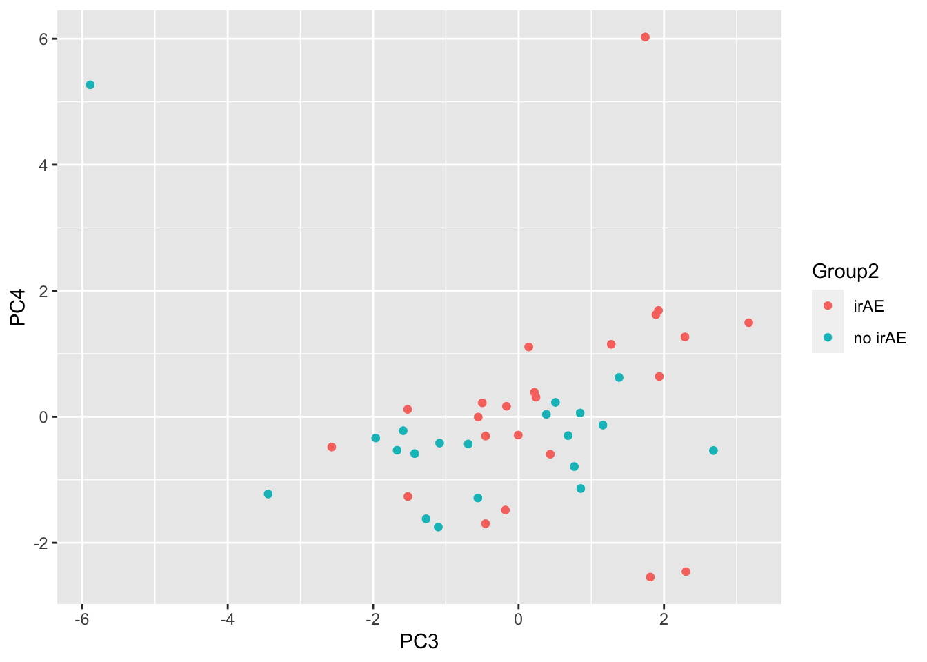

Any PC separate different group?

testTab <- pcTab %>% select(sampleID, PC1:PC20, Group2) %>%
    pivot_longer(-c(sampleID, Group2)) 
resTab <- group_by(testTab, name) %>% nest() %>%
    mutate(m = map(data, ~aov(lm(value ~ Group2,.)))) %>%
    mutate(res = map(m, broom::tidy)) %>%
    unnest(res) %>%
    filter(term == "Group2") %>% arrange(p.value)
resTab %>% select(name, p.value) %>% filter(p.value <=0.05)

# A tibble: 3 × 2
# Groups:   name [3]
  name  p.value
  <chr>   <dbl>
1 PC3   0.00379
2 PC20  0.0179 
3 PC12  0.0201

ggplot(pcTab, aes(x=PC3, y=PC20, col = Group2)) +
    geom_point()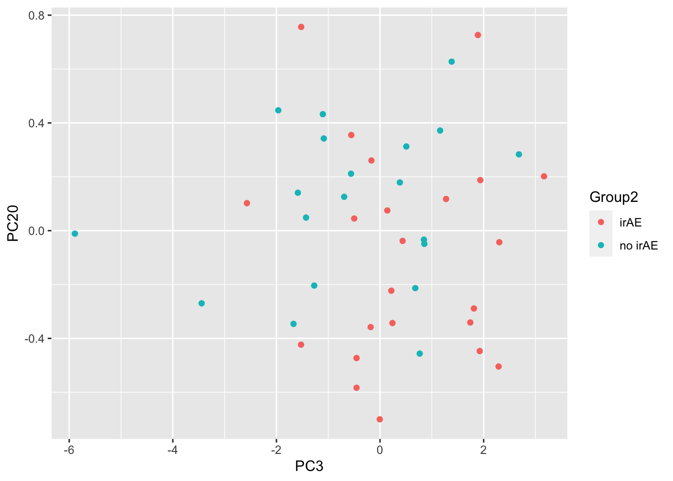

ANOVA

resTab <- subTab %>% group_by(name) %>% nest() %>%
    mutate(m = map(data, ~aov(lm(diffVal ~ Group2,.)))) %>%
    mutate(res = map(m, broom::tidy)) %>%
    unnest(res) %>%
    filter(term == "Group2") %>%
    arrange(p.value) %>%
    select(name, p.value)
resTab.sig <- filter(resTab, p.value < 0.05)
resTab.sig

# A tibble: 3 × 2
# Groups:   name [3]
  name       p.value
  <chr>        <dbl>
1 Choline    0.00564
2 Asparagine 0.0298 
3 Histidine  0.0303

Plot

plotTab <- filter(subTab, name %in% resTab.sig$name)
ggplot(plotTab, aes(x=Group2, y=diffVal)) +
    geom_boxplot(outlier.shape = NA) + ggbeeswarm::geom_quasirandom(aes(col=Group)) +
    facet_wrap(~name, scales = "free")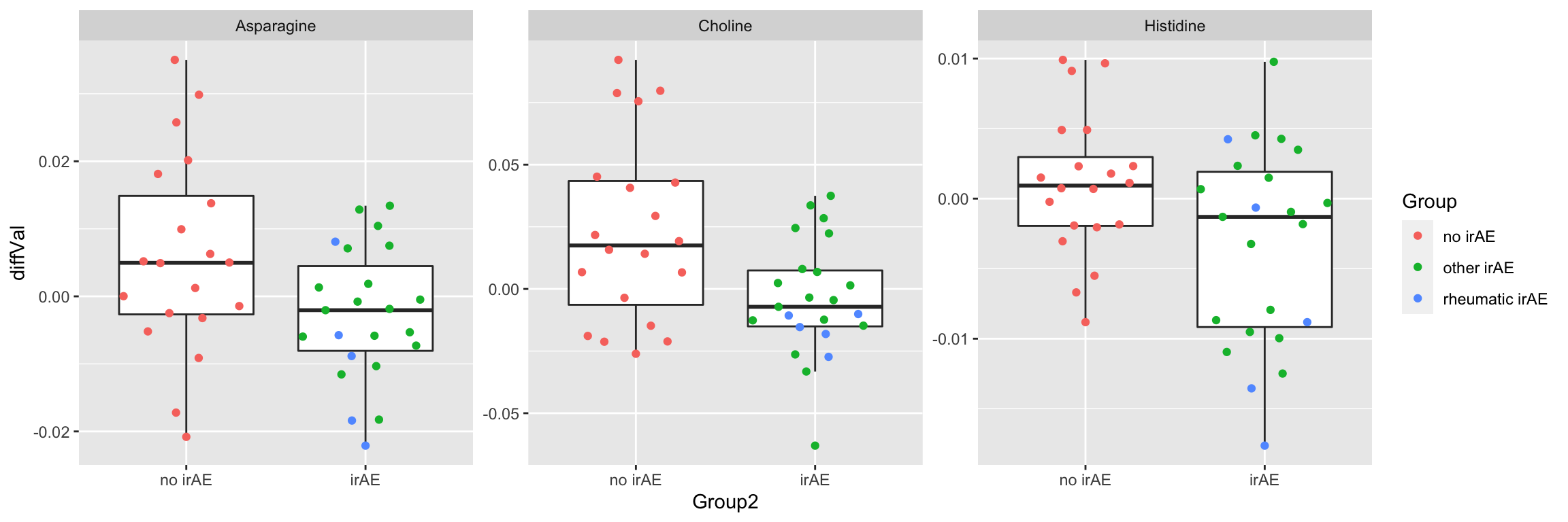

Pair-wise comparison

resPair.diff <- pairwiseT(subTab, "diffVal", "Group2", "name")

Summarise the pariwise comparison results using a heatmap

resPair.cba <- bind_rows(
    resPair.baseline %>% mutate(condition = "Baseline"),
    resPair.followup %>% mutate(condition = "Follow_Up"),
    resPair.diff %>% mutate(condition = "Follow_Up - Baseline")
) 
plotTab <- mutate(resPair.cba, 
                  comparison = paste0(group2, " ~ ", group1),
                  logP = -log10(p.value)*sign(estimate),
                  star = case_when(
                      p.value <= 0.01 ~ "**",
                      p.value <= 0.05 ~ "*",
                      TRUE ~ ""
                  ))

ggplot(plotTab, aes(y=feature, x=comparison)) +
    geom_tile(aes(fill = logP)) +
    geom_text(aes(label = star)) +
    facet_wrap(~condition, ncol=3) +
    theme(axis.text.x = element_text(angle = 90, hjust = 1, vjust = 0.5)) +
    scale_fill_gradient2(low="blue", high="red")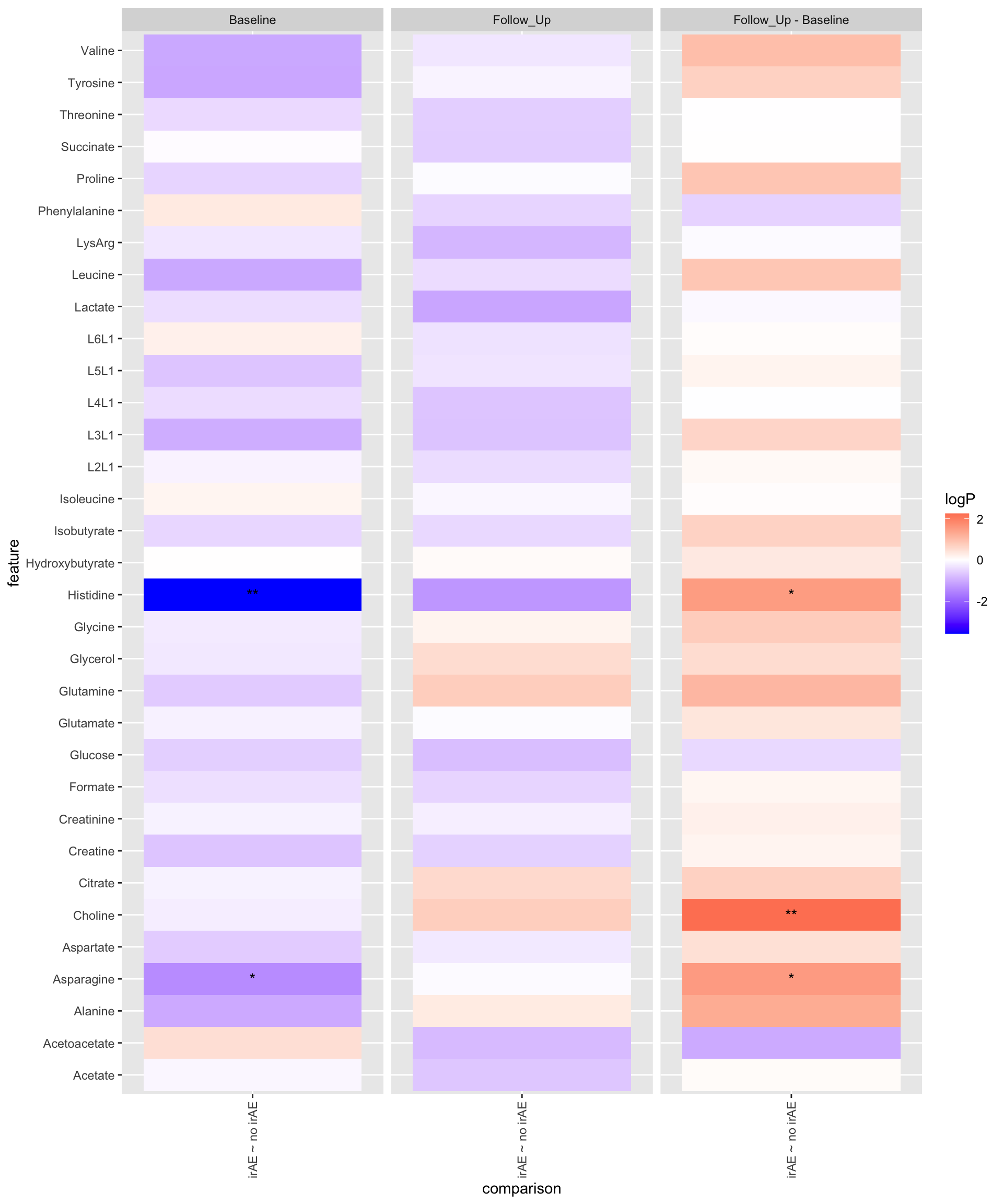

Analysis focused on none-cancer patients

CBA data

cbaTab <- filter(fullTab, assay == "CBA") %>%
    mutate(logVal = glog2(value))

Baseline samples

subTab <- filter(cbaTab, condition == "noMalignancy" )

PCA

subMat <- subTab %>% select(sampleID, name, logVal) %>%
    pivot_wider(names_from = name, values_from = logVal) %>%
    column_to_rownames("sampleID") %>% as.matrix()

pcRes <- prcomp(subMat, center = TRUE, scale. = TRUE)
pcTab <- pcRes$x %>% as_tibble(rownames = "sampleID") %>%
    left_join(patAnno, by = "sampleID")

ggplot(pcTab, aes(x=PC1, y=PC2, col = Group, shape = factor(dateOfAcquisition_CBA))) +
    geom_point()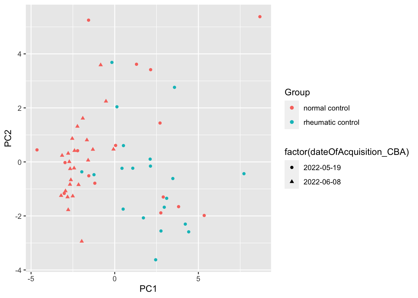

ggplot(pcTab, aes(x=PC3, y=PC4, col = Group, shape = factor(dateOfAcquisition_CBA))) +
    geom_point()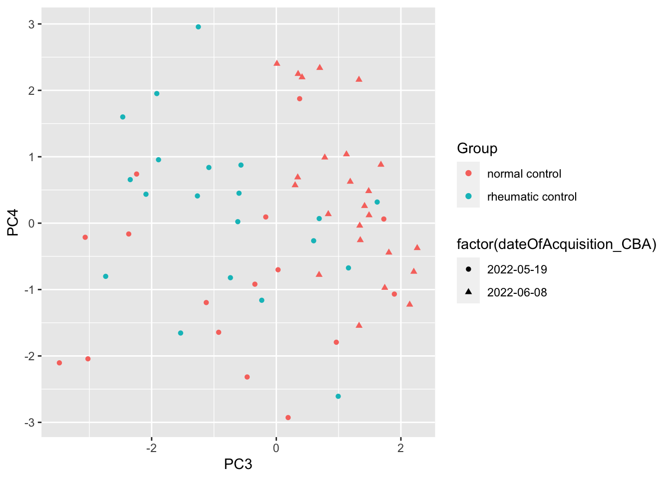

Batch can be a confounder, remove sample with the second batch

subTab <- filter(subTab, as.character(dateOfAcquisition_CBA) != "2022-06-08")
subMat <- subTab %>% 
    select(sampleID, name, logVal) %>%
    pivot_wider(names_from = name, values_from = logVal) %>%
    column_to_rownames("sampleID") %>% as.matrix()

pcRes <- prcomp(subMat, center = TRUE, scale. = TRUE)
pcTab <- pcRes$x %>% as_tibble(rownames = "sampleID") %>%
    left_join(patAnno, by = "sampleID")

ggplot(pcTab, aes(x=PC1, y=PC2, col = Group, shape = factor(dateOfAcquisition_CBA))) +
    geom_point()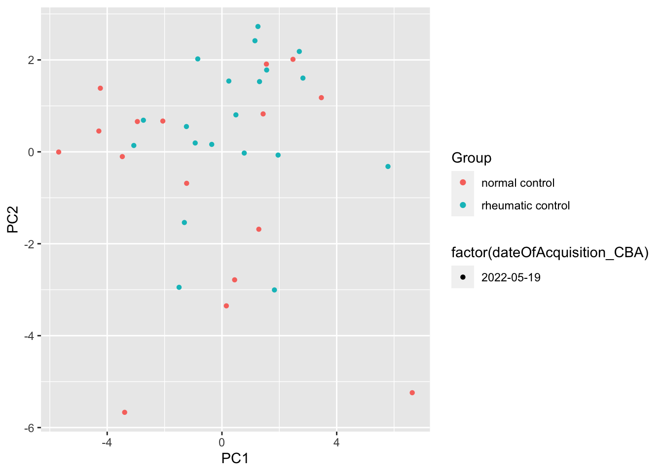

ggplot(pcTab, aes(x=PC3, y=PC4, col = Group, shape = factor(dateOfAcquisition_CBA))) +
    geom_point()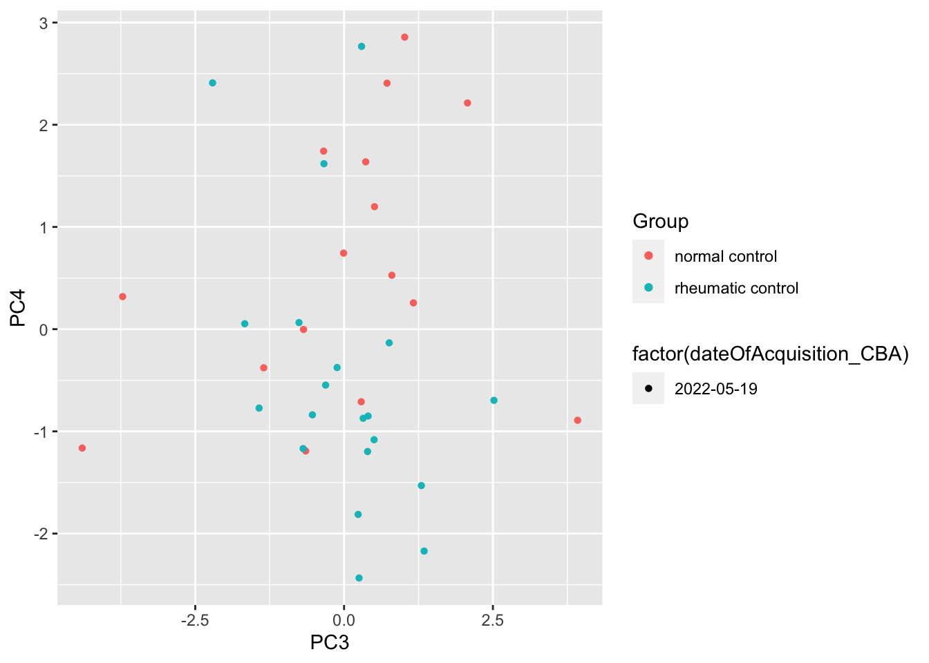

Any PC separate different group?

testTab <- pcTab %>% select(sampleID, PC1:PC20, Group) %>%
    pivot_longer(-c(sampleID, Group)) 
resTab <- group_by(testTab, name) %>% nest() %>%
    mutate(m = map(data, ~aov(lm(value ~ Group,.)))) %>%
    mutate(res = map(m, broom::tidy)) %>%
    unnest(res) %>%
    filter(term == "Group") %>% arrange(p.value)
resTab %>% select(name, p.value) %>% filter(p.value <=0.05)

# A tibble: 1 × 2
# Groups:   name [1]
  name  p.value
  <chr>   <dbl>
1 PC4    0.0222

ggplot(pcTab, aes(x=PC1, y=PC4, col = Group, shape = factor(dateOfAcquisition_CBA))) +
    geom_point()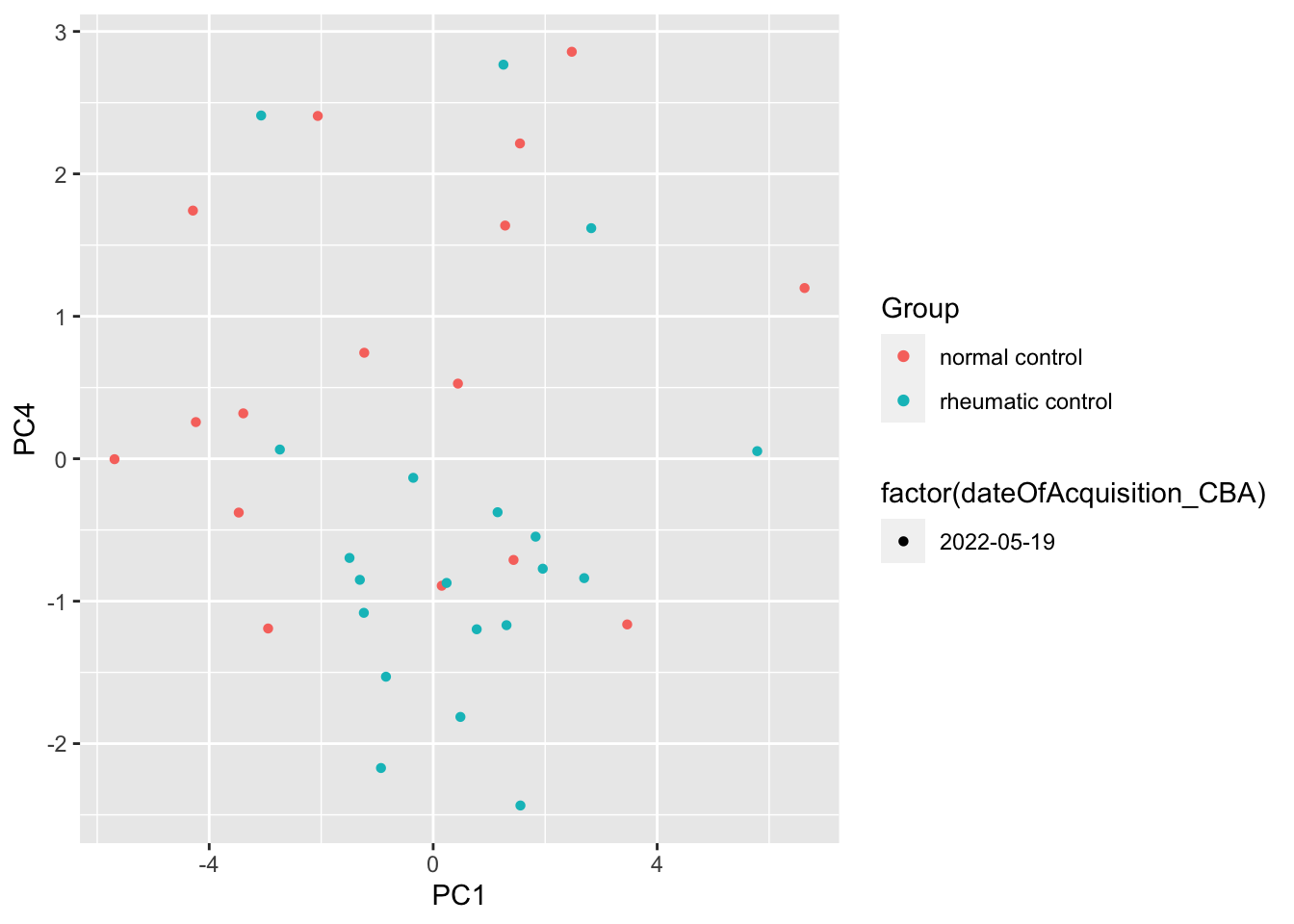

ANOVA

resTab <- subTab %>% group_by(name) %>% nest() %>%
    mutate(m = map(data, ~car::Anova(lm(logVal ~ Group,.)))) %>%
    mutate(res = map(m, broom::tidy)) %>%
    unnest(res) %>%
    filter(term == "Group") %>%
    arrange(p.value) %>%
    select(name, p.value)
resTab.sig <- filter(resTab, p.value < 0.05)
resTab.sig

# A tibble: 3 × 2
# Groups:   name [3]
  name     p.value
  <chr>      <dbl>
1 IL-12p70  0.0317
2 sCD40L    0.0456
3 IL-33     0.0458

Plot

plotTab <- filter(subTab, name %in% resTab.sig$name)
ggplot(plotTab, aes(x=Group, y=logVal)) +
    geom_boxplot(outlier.shape = NA) + ggbeeswarm::geom_quasirandom(aes(col = Group)) +
    facet_wrap(~name, scales = "free")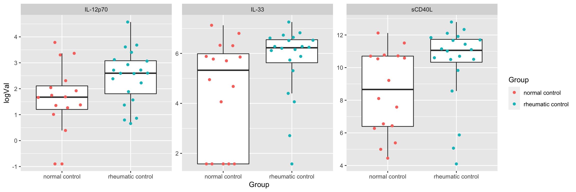

NMR data

nmrTab <- filter(fullTab, assay == "NMR") %>%
    mutate(logVal = value)

Try vsn transformation

nmrMat <- assays(mae)[["nmr"]]
#vsnFit <- vsn::vsnMatrix(nmrMat, minDataPointsPerStratum = 10)
#nmrMat <- predict(vsnFit, nmrMat)
vsnTab <- nmrMat %>% as_tibble(rownames = "name") %>%
    pivot_longer(-name, names_to = "sampleID", values_to = "logVal")
#nmrTab <- left_join(nmrTab, vsnTab, by =c("sampleID","name"))

Baseline samples

subTab <- filter(nmrTab, condition == "noMalignancy" )

PCA

subMat <- subTab %>% select(sampleID, name, logVal) %>%
    pivot_wider(names_from = name, values_from = logVal) %>%
    column_to_rownames("sampleID") %>% as.matrix()

pcRes <- prcomp(subMat, center = TRUE, scale. = TRUE)
pcTab <- pcRes$x %>% as_tibble(rownames = "sampleID") %>%
    left_join(patAnno, by = "sampleID")

ggplot(pcTab, aes(x=PC1, y=PC2, col = Group)) +
    geom_point()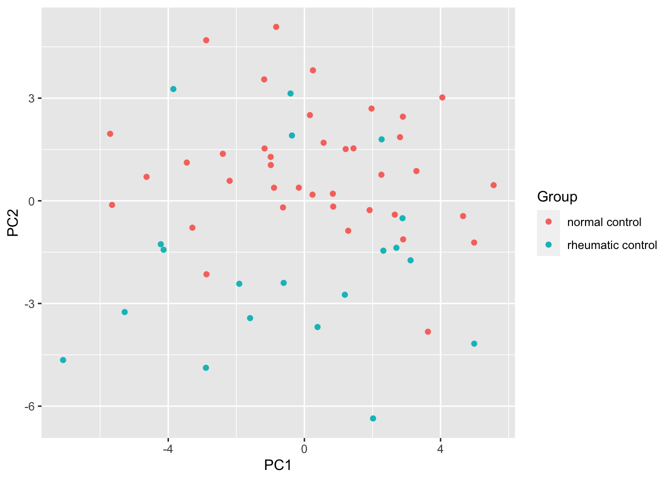

ggplot(pcTab, aes(x=PC3, y=PC4, col = Group)) +
    geom_point()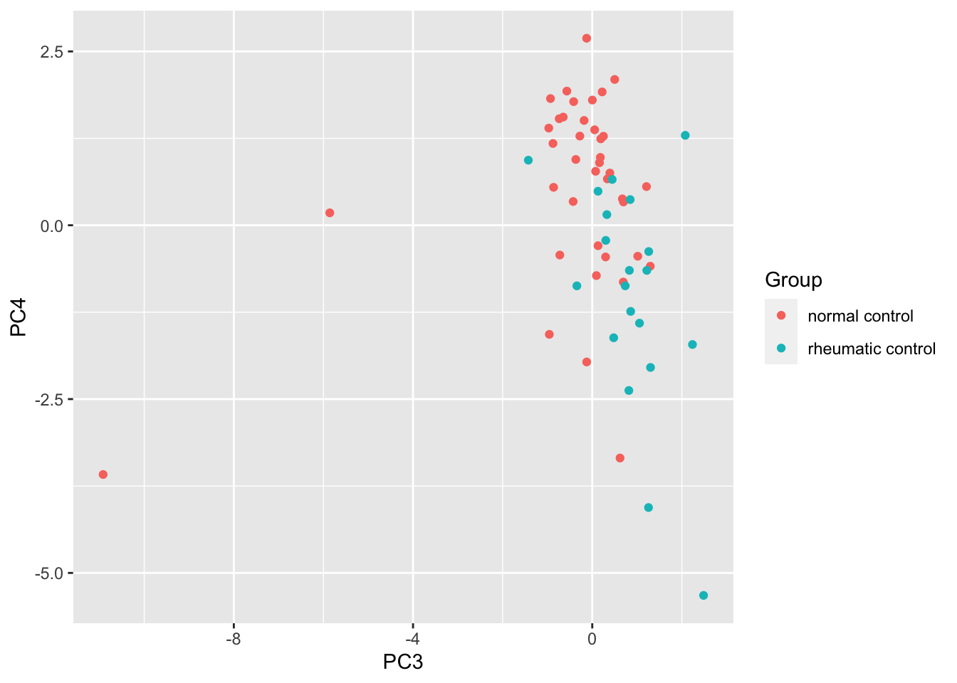

Any PC separate different group?

testTab <- pcTab %>% select(sampleID, PC1:PC20, Group) %>%
    pivot_longer(-c(sampleID, Group)) 
resTab <- group_by(testTab, name) %>% nest() %>%
    mutate(m = map(data, ~aov(lm(value ~ Group,.)))) %>%
    mutate(res = map(m, broom::tidy)) %>%
    unnest(res) %>%
    filter(term == "Group") %>% arrange(p.value)
resTab %>% select(name, p.value) %>% filter(p.value <=0.05)

# A tibble: 3 × 2
# Groups:   name [3]
  name    p.value
  <chr>     <dbl>
1 PC2   0.0000203
2 PC4   0.000605 
3 PC3   0.0103

ggplot(pcTab, aes(x=PC2, y=PC4, col = Group)) +
    geom_point()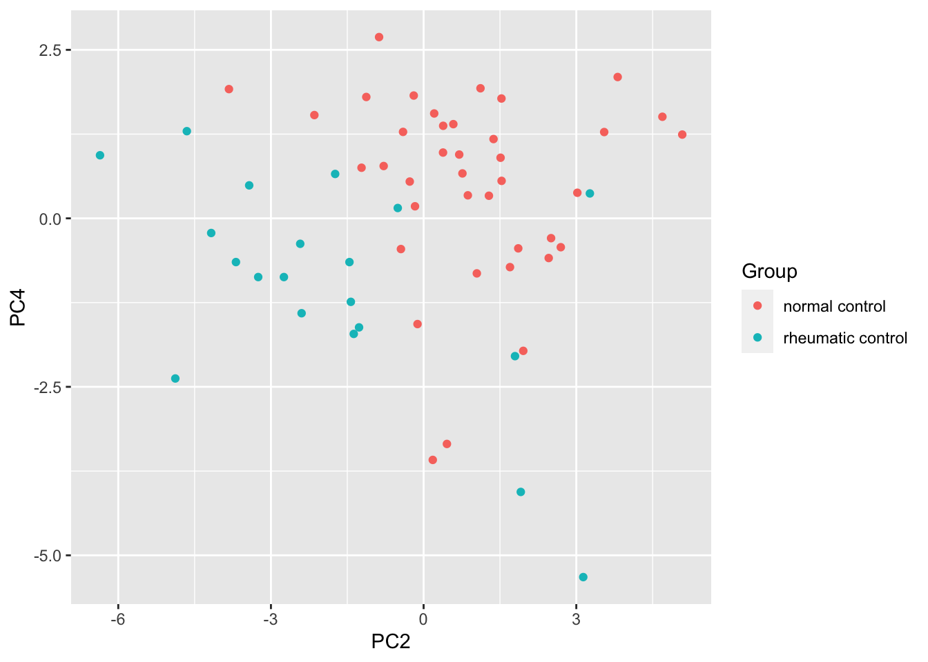

ANOVA

resTab <- subTab %>% group_by(name) %>% nest() %>%
    mutate(m = map(data, ~aov(lm(logVal ~ Group,.)))) %>%
    mutate(res = map(m, broom::tidy)) %>%
    unnest(res) %>%
    filter(term == "Group") %>%
    arrange(p.value) %>%
    select(name, p.value)
resTab.sig <- filter(resTab, p.value < 0.05)
resTab.sig

# A tibble: 9 × 2
# Groups:   name [9]
  name                  p.value
  <chr>                   <dbl>
1 Asparagine      0.00000000158
2 Histidine       0.0000000241 
3 L2L1            0.00000152   
4 L6L1            0.00000904   
5 Aspartate       0.0000500    
6 Lactate         0.000381     
7 Creatine        0.000594     
8 L4L1            0.00429      
9 Hydroxybutyrate 0.0125

Plot

plotTab <- filter(subTab, name %in% resTab.sig$name)
ggplot(plotTab, aes(x=Group, y=logVal)) +
    geom_boxplot() + geom_point() +
    facet_wrap(~name, scales = "free")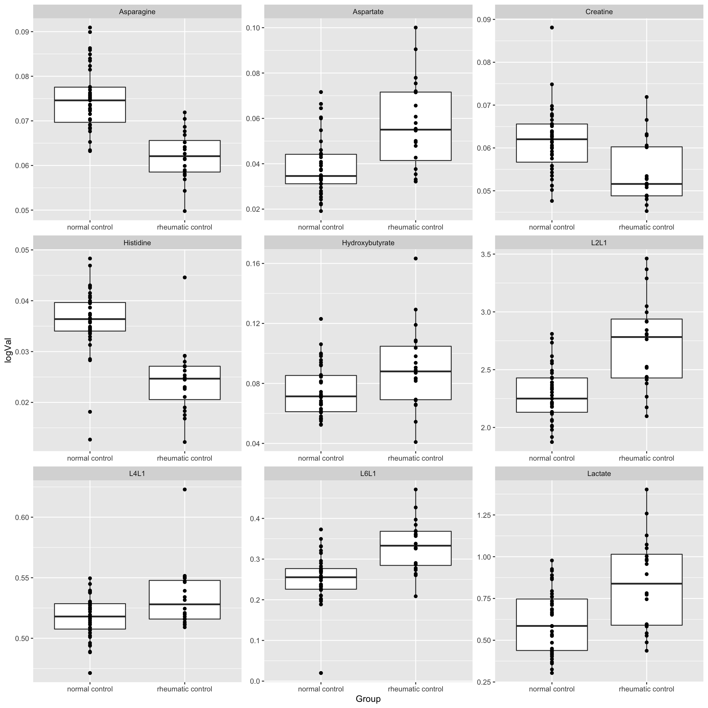

Compare follow-up sample to baseline samples in cancer patients

CBA data

cbaTab <- filter(fullTab, assay == "CBA") %>%
  mutate(logVal = glog2(value)) %>%
  mutate(Group = factor(Group, levels = c("no irAE","rheumatic irAE","other irAE"))) %>%
  filter(Group != "noMalignancy")

testTab <- cbaTab %>% select(name, logVal, condition, Group, patID) %>%
  pivot_wider(names_from = condition, values_from = logVal) %>%
  filter(!is.na(Baseline), !is.na(Follow_Up))
resTab <- group_by(testTab, name, Group) %>% nest() %>%
  mutate(m = map(data, ~t.test(.$Baseline, .$Follow_Up, paired = TRUE))) %>%
  mutate(res = map(m, broom::tidy)) %>%
  unnest(res) %>% select(name,Group, estimate, p.value) %>%
  arrange(p.value)

P-value heatmap

plotTab <- mutate(resTab, 
                  logP = -log10(p.value)*sign(estimate),
                  star = case_when(
                      p.value <= 0.01 ~ "**",
                      p.value <= 0.05 ~ "*",
                      TRUE ~ ""
                  ))

ggplot(plotTab, aes(y=Group, x=name)) +
    geom_tile(aes(fill = logP)) +
    geom_text(aes(label = star)) +
    theme(axis.text.x = element_text(angle = 90, hjust = 1, vjust = 0.5)) +
    scale_fill_gradient2(low="blue", high="red")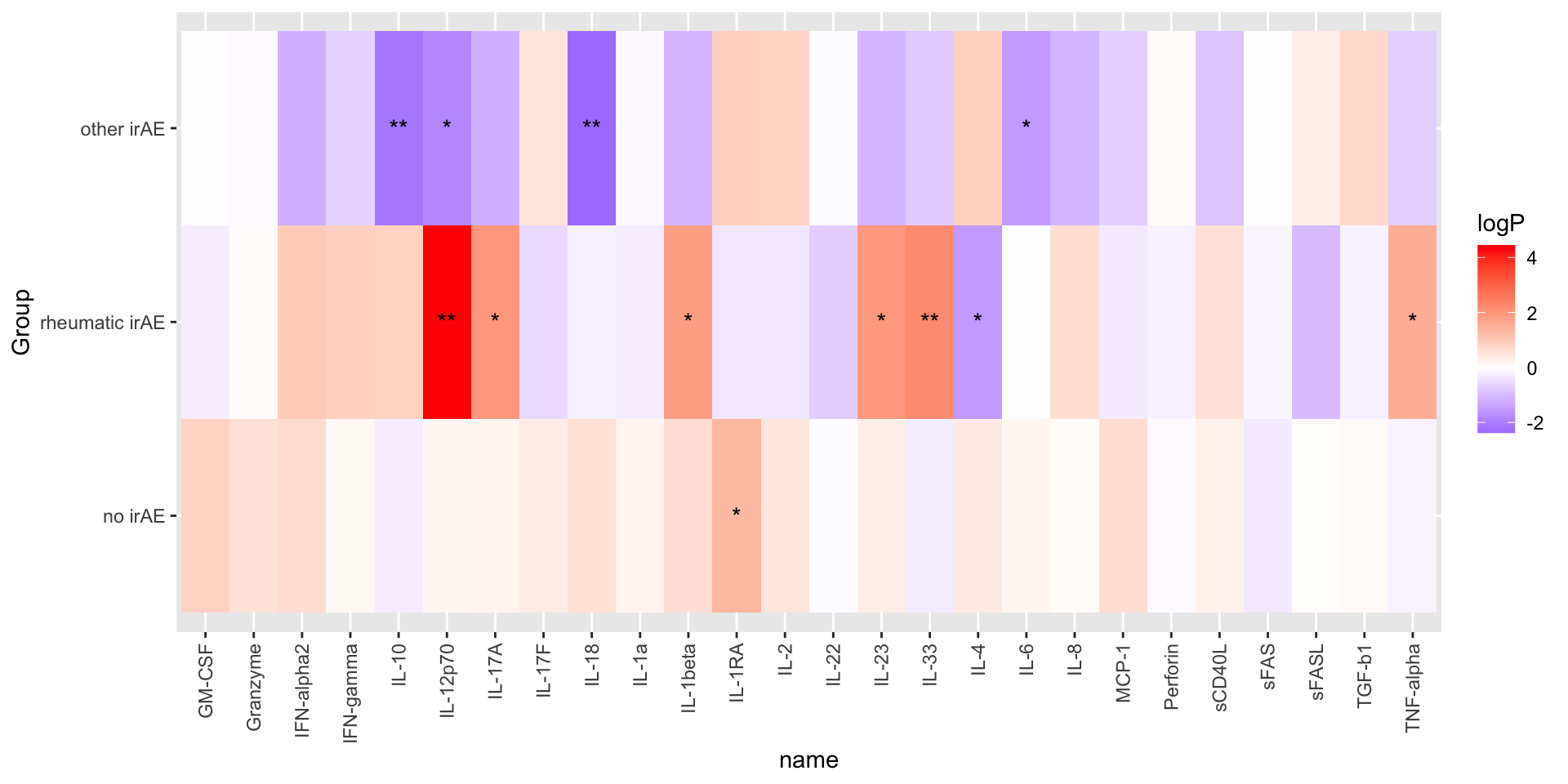

Plot individual associations

resTab.sig <- filter(resTab, p.value <=0.05)
pList <- lapply(unique(resTab.sig$name), function(nn) {
  pTab <- filter(resTab, name ==nn)
  plotTab <- filter(cbaTab, name ==nn) %>%
    left_join(pTab, by = c("name","Group")) %>%
    mutate(title = sprintf("%s (%s)", Group, formatC(p.value, digits = 2)))
  
  ggplot(plotTab, aes(x=condition, y=logVal, col = title)) +
    geom_point() +
    geom_line(aes(group=patID), linetype = "dotted") +
    facet_wrap(~title) + ggtitle(nn) +
    theme_bw() +
    theme(plot.title = element_text(face="bold", hjust = 0.5),
          legend.position = "none")
})
cowplot::plot_grid(plotlist = pList, ncol=2)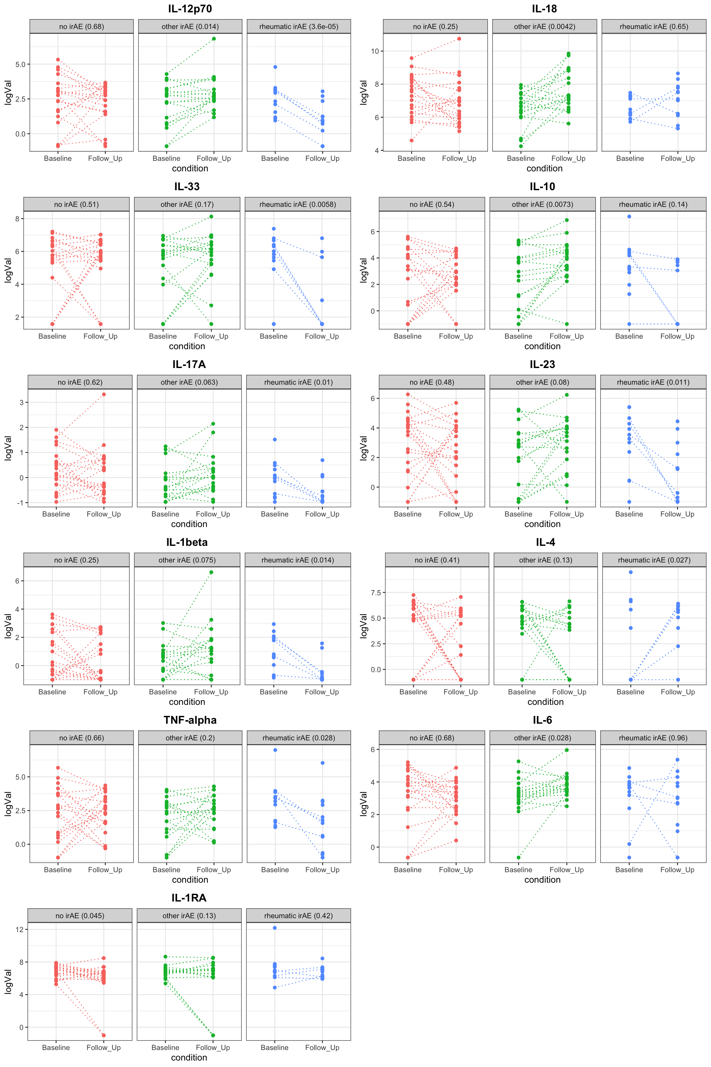

NMR data

cbaTab <- filter(fullTab, assay == "NMR") %>%
  mutate(logVal = value) %>%
  mutate(Group = factor(Group, levels = c("no irAE","rheumatic irAE","other irAE"))) %>%
  filter(Group != "noMalignancy")

testTab <- cbaTab %>% select(name, logVal, condition, Group, patID) %>%
  pivot_wider(names_from = condition, values_from = logVal) %>%
  filter(!is.na(Baseline), !is.na(Follow_Up))
resTab <- group_by(testTab, name, Group) %>% nest() %>%
  mutate(m = map(data, ~t.test(.$Baseline, .$Follow_Up, paired = TRUE))) %>%
  mutate(res = map(m, broom::tidy)) %>%
  unnest(res) %>% select(name,Group, estimate, p.value) %>%
  arrange(p.value)

P-value heatmap

plotTab <- mutate(resTab, 
                  logP = -log10(p.value)*sign(estimate),
                  star = case_when(
                      p.value <= 0.01 ~ "**",
                      p.value <= 0.05 ~ "*",
                      TRUE ~ ""
                  ))

ggplot(plotTab, aes(y=Group, x=name)) +
    geom_tile(aes(fill = logP)) +
    geom_text(aes(label = star)) +
    theme(axis.text.x = element_text(angle = 90, hjust = 1, vjust = 0.5)) +
    scale_fill_gradient2(low="blue", high="red")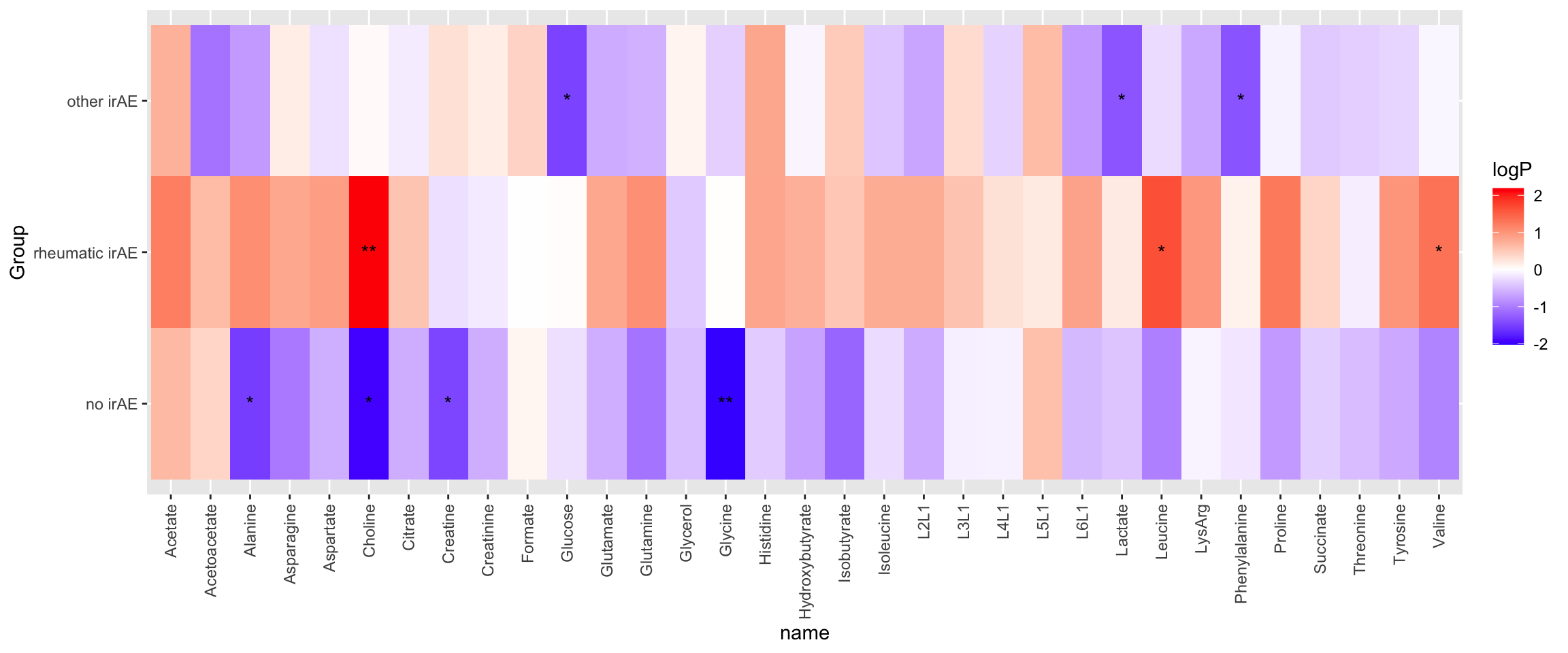

Plot individual associations

resTab.sig <- filter(resTab, p.value <=0.05)
pList <- lapply(unique(resTab.sig$name), function(nn) {
  pTab <- filter(resTab, name ==nn)
  plotTab <- filter(cbaTab, name ==nn) %>%
    left_join(pTab, by = c("name","Group")) %>%
    mutate(title = sprintf("%s (%s)", Group, formatC(p.value, digits = 2)))
  
  ggplot(plotTab, aes(x=condition, y=logVal, col = title)) +
    geom_point() +
    geom_line(aes(group=patID), linetype = "dotted") +
    facet_wrap(~title) + ggtitle(nn) +
    theme_bw() +
    theme(plot.title = element_text(face="bold", hjust = 0.5),
          legend.position = "none")
})
cowplot::plot_grid(plotlist = pList, ncol=2)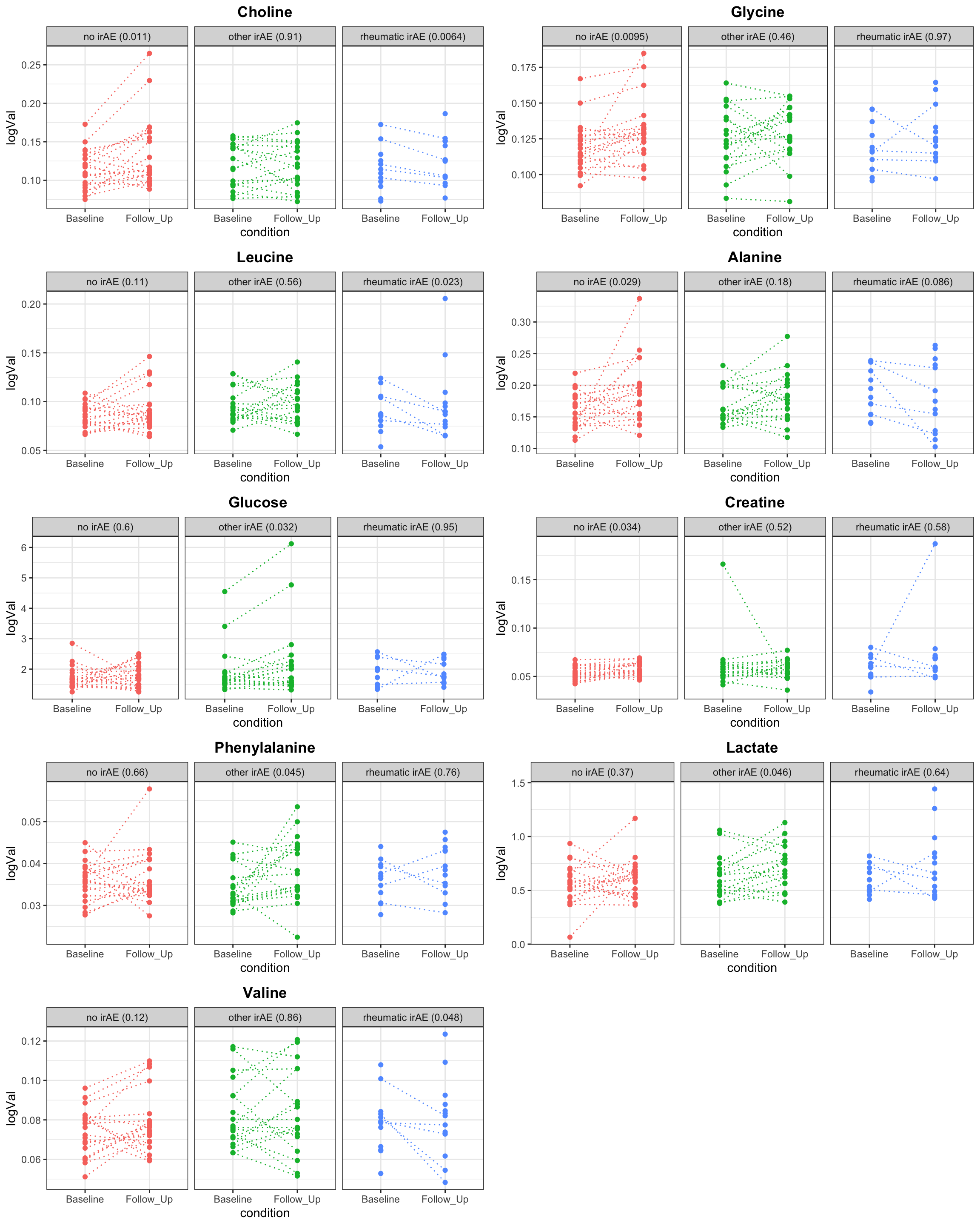

Healthy controls vs baseline of all cancer groups

CBA data

Remove one batch to avoid batch effect

testTab <- filter(fullTab, assay == "CBA", as.character(dateOfAcquisition_CBA) != "2022-06-08") %>%
  mutate(logVal = glog2(value)) %>%
  filter(Group !="rheumatic control", condition %in% c("Baseline","noMalignancy")) %>%
  mutate(testGroup = ifelse(condition == "Baseline", "cancer", "healthy"))

Test results

resTab <- group_by(testTab, name) %>% nest() %>%
  mutate(m = map(data, ~t.test(logVal ~ testGroup, var.equal=TRUE, data = .))) %>%
  mutate(res = map(m, broom::tidy)) %>%
  unnest(res) %>% select(name, estimate, p.value) %>%
  arrange(p.value)

resTab.sig <- filter(resTab, p.value <= 0.05)
resTab.sig

# A tibble: 3 × 3
# Groups:   name [3]
  name       estimate p.value
  <chr>         <dbl>   <dbl>
1 sCD40L        1.85  0.00190
2 GM-CSF        0.988 0.0269 
3 IFN-alpha2    0.645 0.0427

Plot significant associations (p<=0.05)

resTab.sig <- filter(resTab, p.value <=0.05)

plotTab <- filter(testTab, name %in% resTab.sig$name)
  
ggplot(plotTab, aes(x=testGroup, y=logVal)) +
  geom_boxplot(outlier.shape = NA) +
  ggbeeswarm::geom_quasirandom(aes(col = Group)) +
  theme_bw() +
  theme(plot.title = element_text(face="bold", hjust = 0.5),
        legend.position = "bottom") +
  facet_wrap(~name, scales = "free")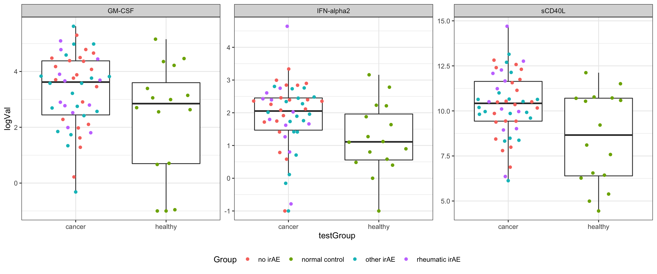

NMR data

testTab <- filter(fullTab, assay == "NMR") %>%
  mutate(logVal = value) %>%
  filter(Group !="rheumatic control", condition %in% c("Baseline","noMalignancy")) %>%
  mutate(testGroup = ifelse(condition == "Baseline", "cancer", "healthy"))

Test results

resTab <- group_by(testTab, name) %>% nest() %>%
  mutate(m = map(data, ~t.test(logVal ~ testGroup, var.equal=TRUE, data = .))) %>%
  mutate(res = map(m, broom::tidy)) %>%
  unnest(res) %>% select(name, estimate, p.value) %>%
  arrange(p.value)

resTab.sig <- filter(resTab, p.value <= 0.01)
resTab.sig

# A tibble: 23 × 3
# Groups:   name [23]
   name      estimate  p.value
   <chr>        <dbl>    <dbl>
 1 Glutamine  0.0728  2.07e-23
 2 Histidine -0.0167  2.23e-21
 3 L6L1       0.126   3.54e-20
 4 Succinate -0.00474 1.32e-17
 5 Choline    0.0478  2.15e-14
 6 Aspartate  0.0319  2.06e-13
 7 L3L1      -0.0765  3.36e-13
 8 L2L1       0.417   2.32e-12
 9 Glutamate -0.0451  3.58e-12
10 Formate   -0.00335 3.44e- 9
# … with 13 more rows
# ℹ Use `print(n = ...)` to see more rows

Plot significant associations (p<=0.01)

plotTab <- filter(testTab, name %in% resTab.sig$name)
  
ggplot(plotTab, aes(x=testGroup, y=logVal)) +
  geom_boxplot(outlier.shape = NA) +
  ggbeeswarm::geom_quasirandom(aes(col = Group)) +
  theme_bw() +
  theme(plot.title = element_text(face="bold", hjust = 0.5),
        legend.position = "bottom") +
  facet_wrap(~name, scales = "free", ncol = 3)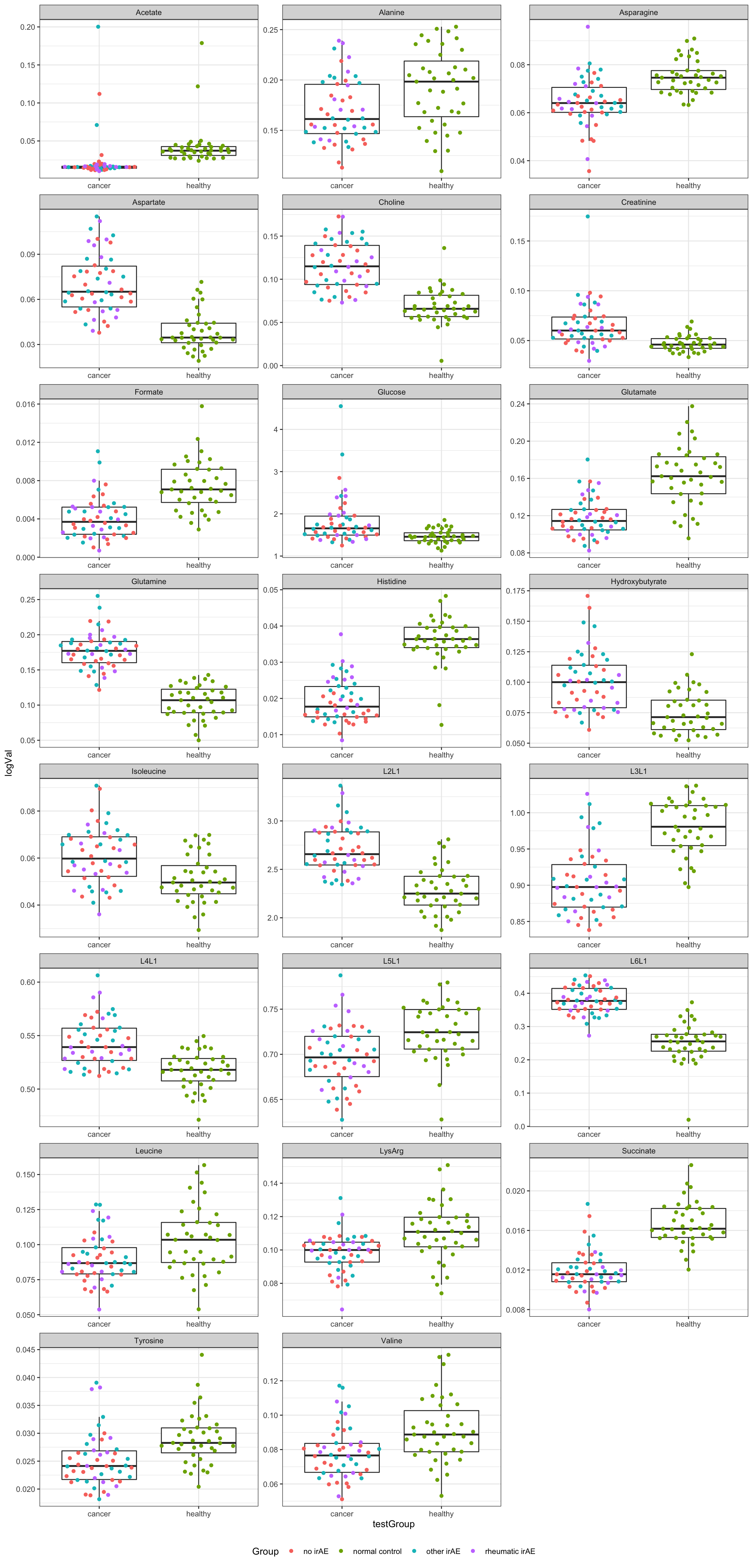

Rheuma irAE at follow-up vs Rheumatic non-cancer

CBA data

Remove one batch to avoid batch effect

testTab <- filter(fullTab, assay == "CBA", as.character(dateOfAcquisition_CBA) != "2022-06-08") %>%
  mutate(logVal = glog2(value)) %>%
  filter(Group %in% c("rheumatic control","rheumatic irAE"), condition %in% c("Follow_Up","noMalignancy"))

resTab <- group_by(testTab, name) %>% nest() %>%
  mutate(m = map(data, ~t.test(logVal ~ Group, var.equal=TRUE, data = .))) %>%
  mutate(res = map(m, broom::tidy)) %>%
  unnest(res) %>% select(name, estimate, p.value) %>%
  arrange(p.value)

resTab.sig <- filter(resTab, p.value <= 0.05)
resTab.sig

# A tibble: 11 × 3
# Groups:   name [11]
   name      estimate   p.value
   <chr>        <dbl>     <dbl>
 1 IL-33        2.96  0.0000255
 2 IL-12p70     1.72  0.000301 
 3 IL-23        2.09  0.00161  
 4 IL-10        2.28  0.00165  
 5 Perforin    -0.648 0.00248  
 6 IL-8         1.87  0.00736  
 7 TGF-b1      -1.32  0.00787  
 8 IL-17A       0.531 0.0160   
 9 IFN-gamma    0.795 0.0338   
10 GM-CSF      -1.06  0.0449   
11 TNF-alpha    1.13  0.0492

Plot significant associations (p<=0.05)

plotTab <- filter(testTab, name %in% resTab.sig$name)
  
ggplot(plotTab, aes(x=Group, y=logVal)) +
  geom_boxplot(outlier.shape = NA) +
  ggbeeswarm::geom_quasirandom(aes(col = Group)) +
  theme_bw() +
  theme(plot.title = element_text(face="bold", hjust = 0.5),
        legend.position = "bottom") +
  facet_wrap(~name, scales = "free")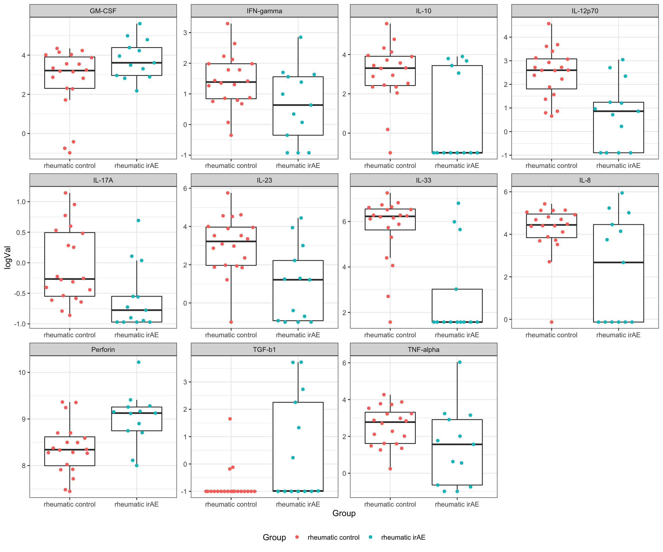

NMR data

Remove one batch to avoid batch effect

testTab <- filter(fullTab, assay == "NMR") %>%
  mutate(logVal = glog2(value)) %>%
  filter(Group %in% c("rheumatic control","rheumatic irAE"), condition %in% c("Follow_Up","noMalignancy"))

resTab <- group_by(testTab, name) %>% nest() %>%
  mutate(m = map(data, ~t.test(logVal ~ Group, var.equal=TRUE, data = .))) %>%
  mutate(res = map(m, broom::tidy)) %>%
  unnest(res) %>% select(name, estimate, p.value) %>%
  arrange(p.value)

resTab.sig <- filter(resTab, p.value <= 0.05)
resTab.sig

# A tibble: 15 × 3
# Groups:   name [15]
   name       estimate    p.value
   <chr>         <dbl>      <dbl>
 1 Glutamine  -0.0862  0.00000102
 2 Choline    -0.0673  0.0000236 
 3 Acetate     0.0164  0.000213  
 4 Formate     0.00425 0.000266  
 5 Creatinine -0.0441  0.000782  
 6 L3L1        0.0717  0.00178   
 7 Glucose    -0.313   0.00250   
 8 L6L1       -0.118   0.00383   
 9 Glutamate   0.0509  0.00406   
10 Glycerol   -0.0172  0.00436   
11 Threonine  -0.0308  0.00439   
12 Aspartate  -0.0340  0.0242    
13 Tyrosine    0.00579 0.0294    
14 Creatine   -0.0266  0.0294    
15 Succinate   0.00371 0.0454

Plot significant associations (p<=0.05)

plotTab <- filter(testTab, name %in% resTab.sig$name)
  
ggplot(plotTab, aes(x=Group, y=logVal)) +
  geom_boxplot(outlier.shape = NA) +
  ggbeeswarm::geom_quasirandom(aes(col = Group)) +
  theme_bw() +
  theme(plot.title = element_text(face="bold", hjust = 0.5),
        legend.position = "bottom") +
  facet_wrap(~name, scales = "free")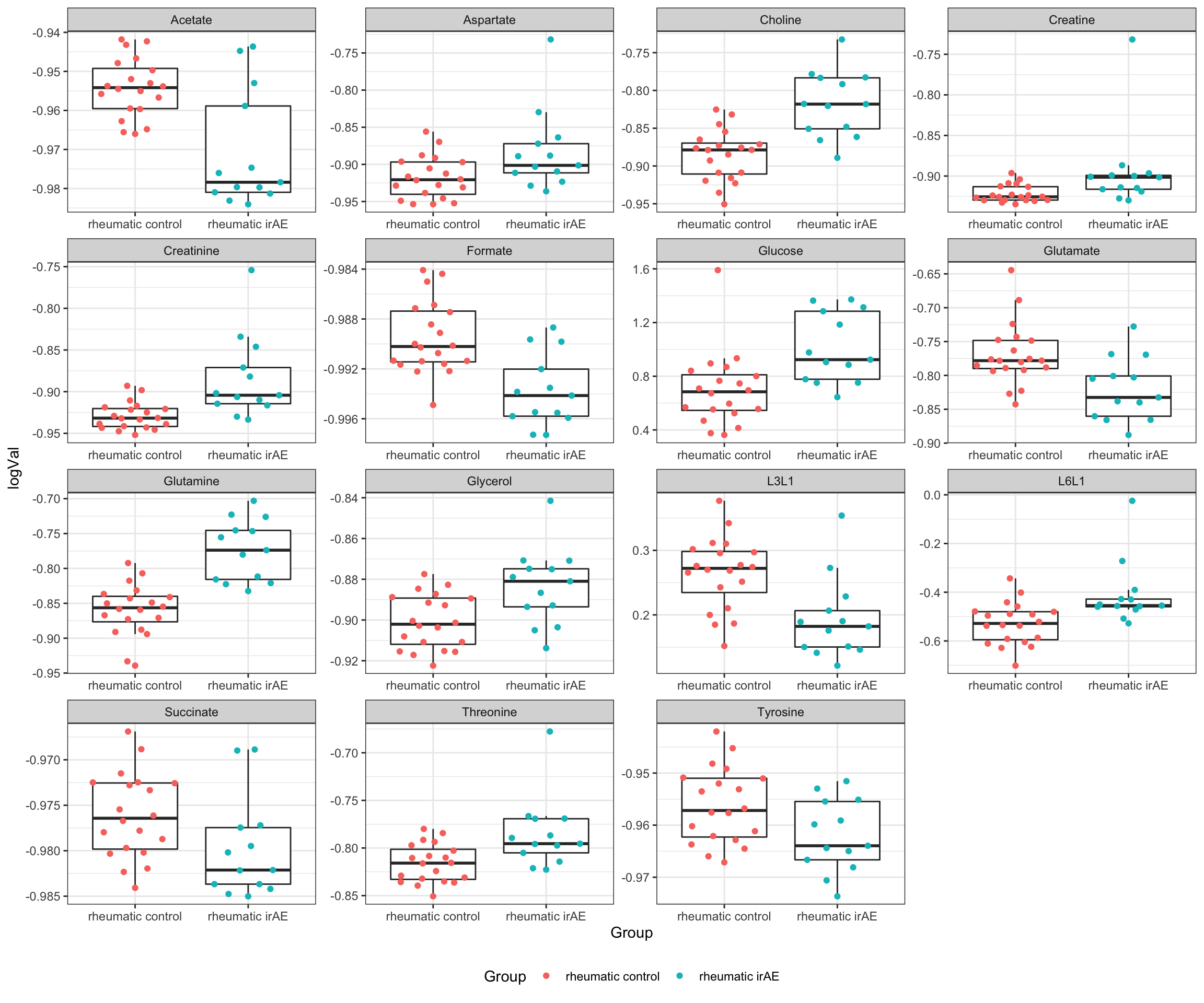

Test for interaction between Cancer and Rheumatic irAE (at follow-up)

CBA data

Remove one batch to avoid batch effect

testTab <- filter(fullTab, assay == "CBA", as.character(dateOfAcquisition_CBA) != "2022-06-08") %>%
  mutate(logVal = glog2(value)) %>%
  filter(Group %in% c("rheumatic control","rheumatic irAE", "normal control", "no irAE"), condition %in% c("Follow_Up","noMalignancy")) %>%
  mutate(cancer = ifelse(condition == "noMalignancy", "noCancer", "withCancer"),
         irAE = ifelse(str_detect(Group, "rheumatic"),"Rheumatic", "noRheumatic")) %>%
  mutate(category = paste0(cancer,"_",irAE))

resTab <- group_by(testTab, name) %>% nest() %>%
  mutate(m = map(data, ~car::Anova(lm(logVal ~cancer+irAE+cancer:irAE,.)))) %>%
  mutate(res = map(m, broom::tidy)) %>%
  unnest(res)

Iteractions between cancer and rheumatic irAE

The below results show the significant interaction between cancer and rheumatic irAE on the molecular profile. A “significant interaction” means the whether the patients have cancer or irAE have non-additive effect, e.g one molecular is up-regulated in patients with irAE in cancer group but down-regulated (or unchanged) in non-cancer group.

resTab.inter <- resTab %>% 
  filter(term == "cancer:irAE") %>%
  select(name, p.value) %>%
  arrange(p.value) %>%
  filter(p.value <= 0.05)
resTab.inter

# A tibble: 9 × 2
# Groups:   name [9]
  name         p.value
  <chr>          <dbl>
1 IL-33      0.0000392
2 IL-12p70   0.000399 
3 IL-10      0.00175  
4 Perforin   0.00587  
5 IL-17A     0.0134   
6 TGF-b1     0.0286   
7 IL-23      0.0340   
8 IFN-gamma  0.0389   
9 IFN-alpha2 0.0482

Plot significant associations (p<=0.05)

plotTab <- filter(testTab, name %in% resTab.inter$name)
  
ggplot(plotTab, aes(x=category, y=logVal)) +
  geom_boxplot(outlier.shape = NA) +
  ggbeeswarm::geom_quasirandom(aes(col = category)) +
  theme_bw() +
  theme(plot.title = element_text(face="bold", hjust = 0.5),
        legend.position = "no",
        axis.text.x = element_text(angle = 90, hjust = 1, vjust = 0)) +
  facet_wrap(~name, scales = "free")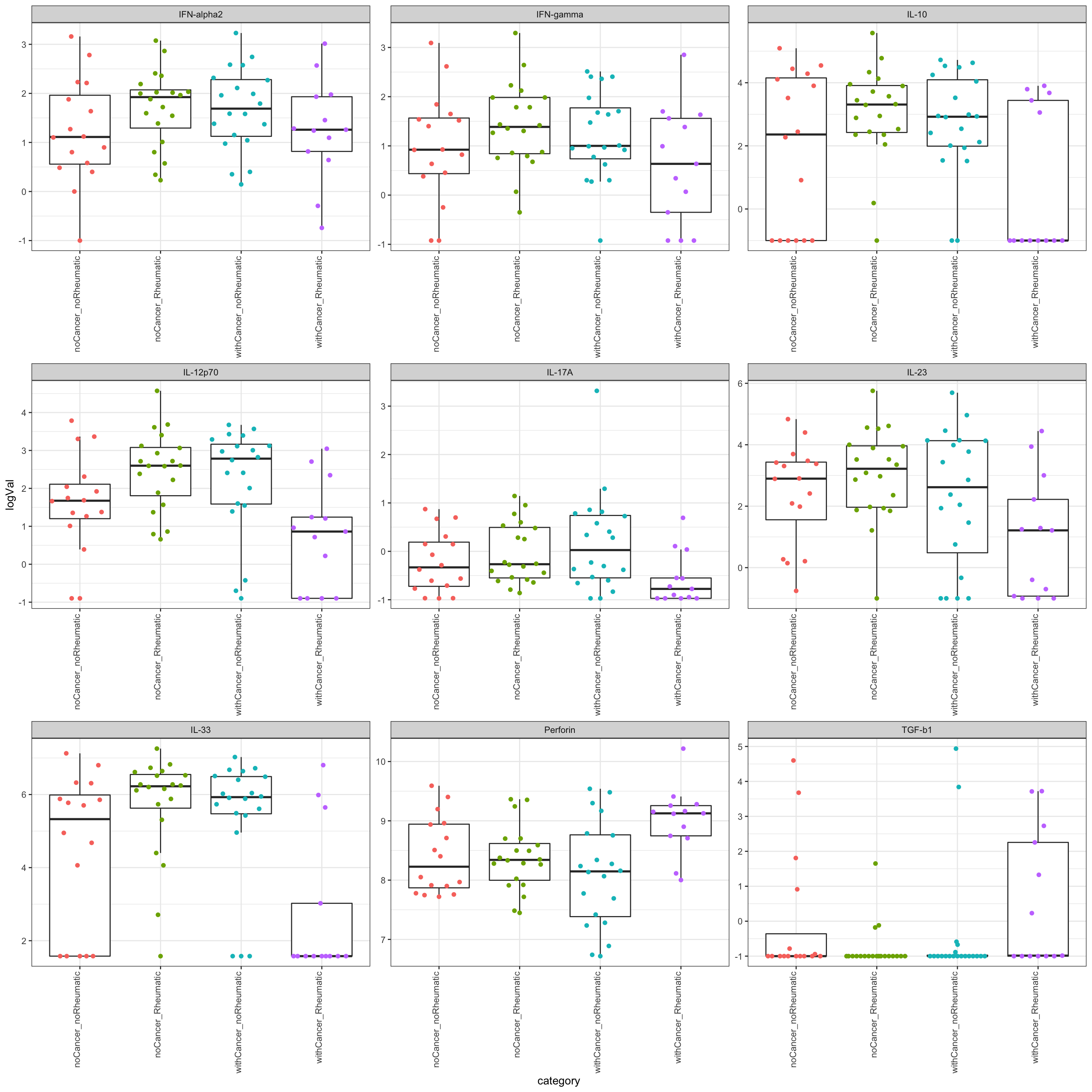

Different between cancer and non-cancer, regardless of irAE status

The below results show the molecules that show similar trend between cancer and non-cancer group, regardless of whether the patients have irAE or not.

resTab.sig <- resTab %>% 
  filter(term == "cancer") %>%
  select(name, p.value) %>%
  arrange(p.value) %>%
  filter(p.value <= 0.05, !name %in% resTab.inter$name)
resTab.sig

# A tibble: 6 × 2
# Groups:   name [6]
  name     p.value
  <chr>      <dbl>
1 Granzyme 0.00220
2 sCD40L   0.0177 
3 IL-8     0.0291 
4 IL-18    0.0421 
5 sFAS     0.0470 
6 GM-CSF   0.0478

Plot significant associations (p<=0.05)

plotTab <- filter(testTab, name %in% resTab.sig$name)
  
ggplot(plotTab, aes(x=cancer, y=logVal)) +
  geom_boxplot(outlier.shape = NA) +
  ggbeeswarm::geom_quasirandom(aes(col = cancer)) +
  theme_bw() +
  theme(plot.title = element_text(face="bold", hjust = 0.5),
        legend.position = "no",
        axis.text.x = element_text(angle = 90, hjust = 1, vjust = 0)) +
  facet_wrap(~name+irAE, scales = "free",ncol=4)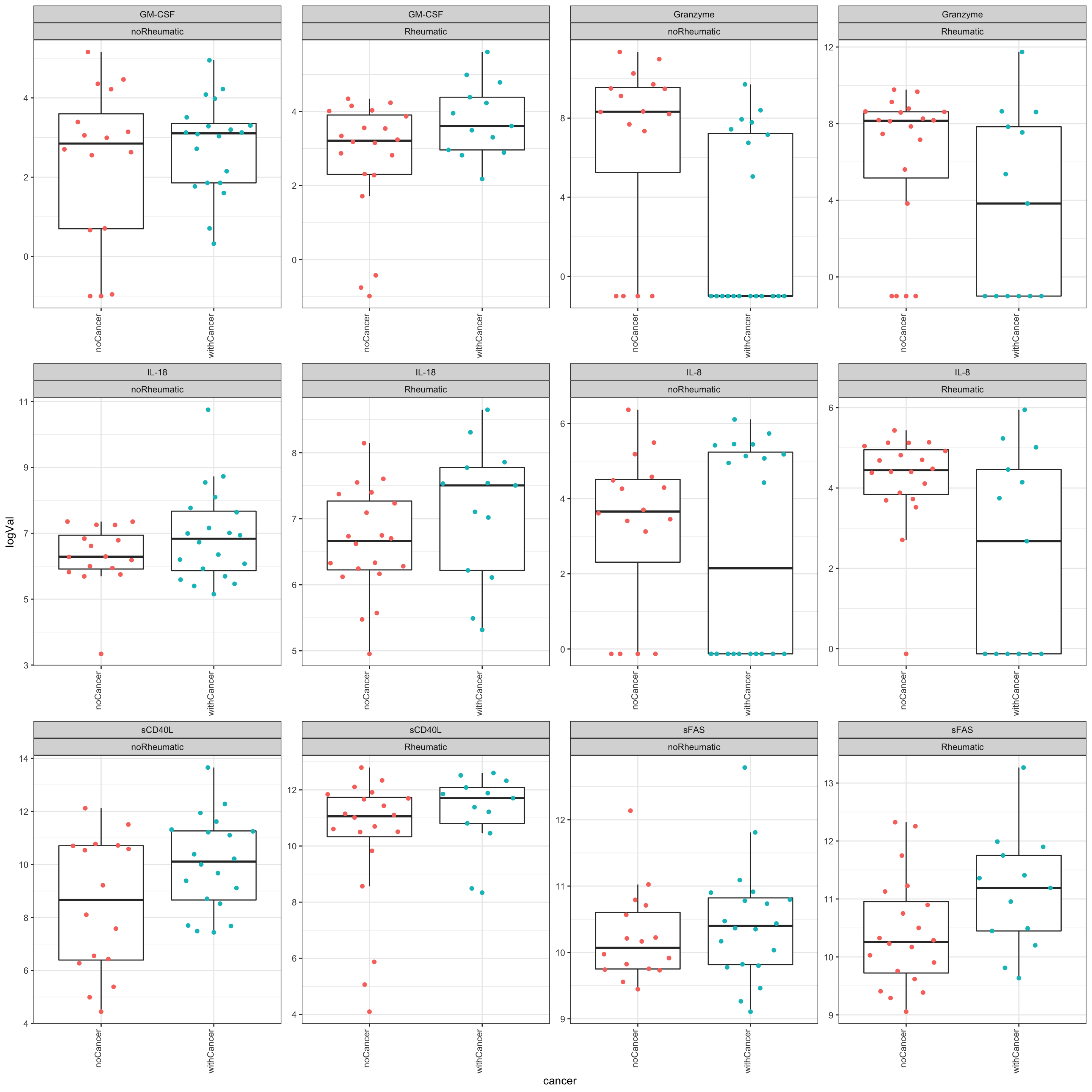

Different between irAE and no irAE, regardless of cancer

The below results show the molecules that show similar trend between rheumatic irAE and non-irAE group, regardless of whether the patients have cancer or not.

resTab.sig <- resTab %>% 
  filter(term == "irAE") %>%
  select(name, p.value) %>%
  arrange(p.value) %>%
  filter(p.value <= 0.05, !name %in% resTab.inter$name)
resTab.sig

# A tibble: 1 × 2
# Groups:   name [1]
  name   p.value
  <chr>    <dbl>
1 sCD40L 0.00623

Plot significant associations (p<=0.05)

plotTab <- filter(testTab, name %in% resTab.sig$name)
  
ggplot(plotTab, aes(x=irAE, y=logVal)) +
  geom_boxplot(outlier.shape = NA) +
  ggbeeswarm::geom_quasirandom(aes(col = irAE)) +
  theme_bw() +
  theme(plot.title = element_text(face="bold", hjust = 0.5),
        legend.position = "no",
        axis.text.x = element_text(angle = 90, hjust = 1, vjust = 0)) +
  facet_wrap(~name+cancer, scales = "free",ncol=4)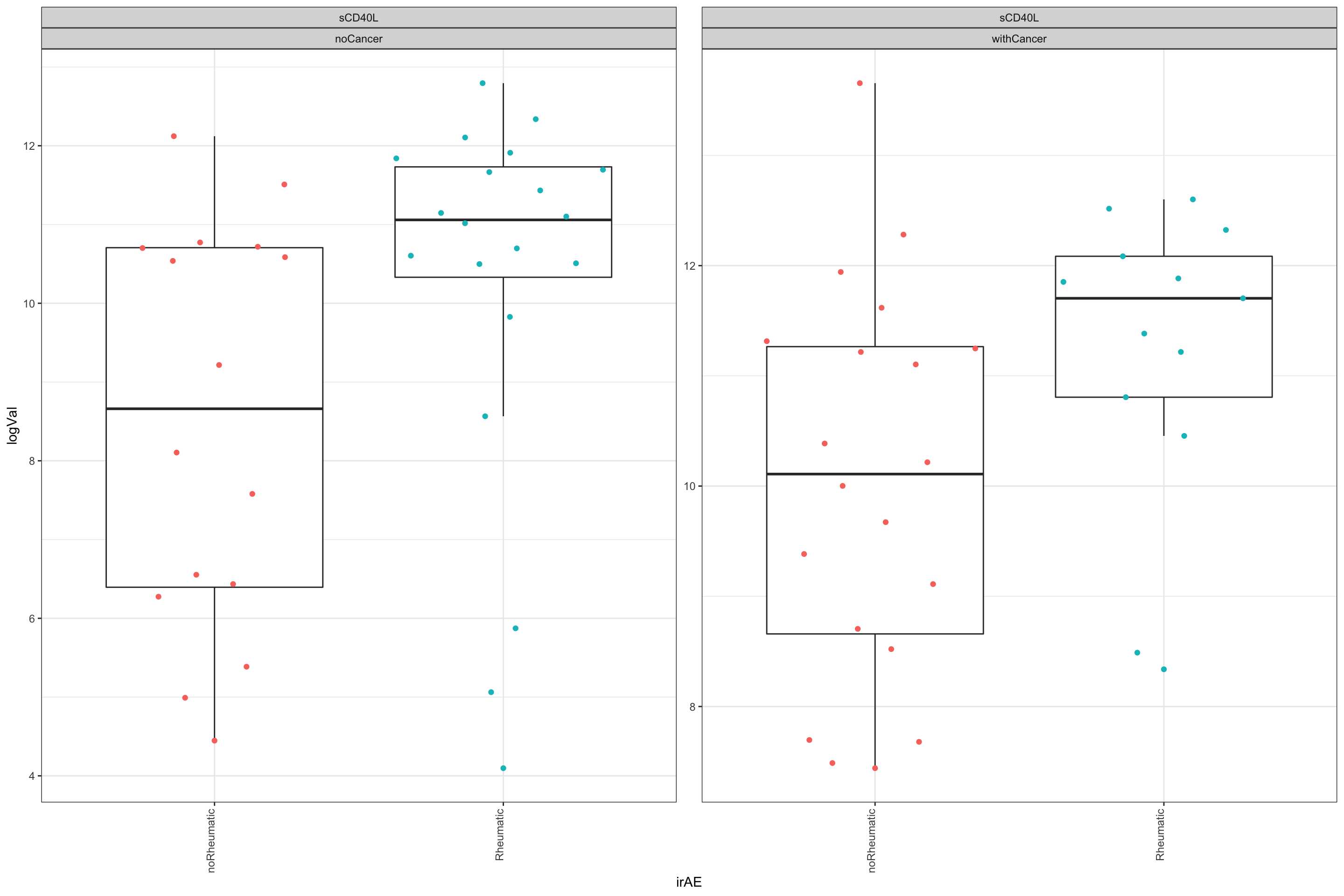

NMR data

The same analyses as for the CBA data.

testTab <- filter(fullTab, assay == "NMR") %>%
  mutate(logVal = glog2(value)) %>%
  filter(Group %in% c("rheumatic control","rheumatic irAE", "normal control", "no irAE"), condition %in% c("Follow_Up","noMalignancy")) %>%
  mutate(cancer = ifelse(condition == "noMalignancy", "noCancer", "withCancer"),
         irAE = ifelse(str_detect(Group, "rheumatic"),"Rheumatic", "noRheumatic")) %>%
  mutate(category = paste0(cancer,"_",irAE))

resTab <- group_by(testTab, name) %>% nest() %>%
  mutate(m = map(data, ~car::Anova(lm(logVal ~cancer+irAE+cancer:irAE,.)))) %>%
  mutate(res = map(m, broom::tidy)) %>%
  unnest(res)

Iteractions between cancer and rheumatic irAE

resTab.inter <- resTab %>% 
  filter(term == "cancer:irAE") %>%
  select(name, p.value) %>%
  arrange(p.value) %>%
  filter(p.value <= 0.05)
resTab.inter

# A tibble: 6 × 2
# Groups:   name [6]
  name            p.value
  <chr>             <dbl>
1 Histidine  0.0000000209
2 Asparagine 0.000616    
3 Creatine   0.000923    
4 L2L1       0.0132      
5 L5L1       0.0359      
6 Glutamine  0.0495

Plot significant associations (p<=0.05)

plotTab <- filter(testTab, name %in% resTab.inter$name)
  
ggplot(plotTab, aes(x=category, y=logVal)) +
  geom_boxplot(outlier.shape = NA) +
  ggbeeswarm::geom_quasirandom(aes(col = category)) +
  theme_bw() +
  theme(plot.title = element_text(face="bold", hjust = 0.5),
        legend.position = "no",
        axis.text.x = element_text(angle = 90, hjust = 1, vjust = 0)) +
  facet_wrap(~name, scales = "free")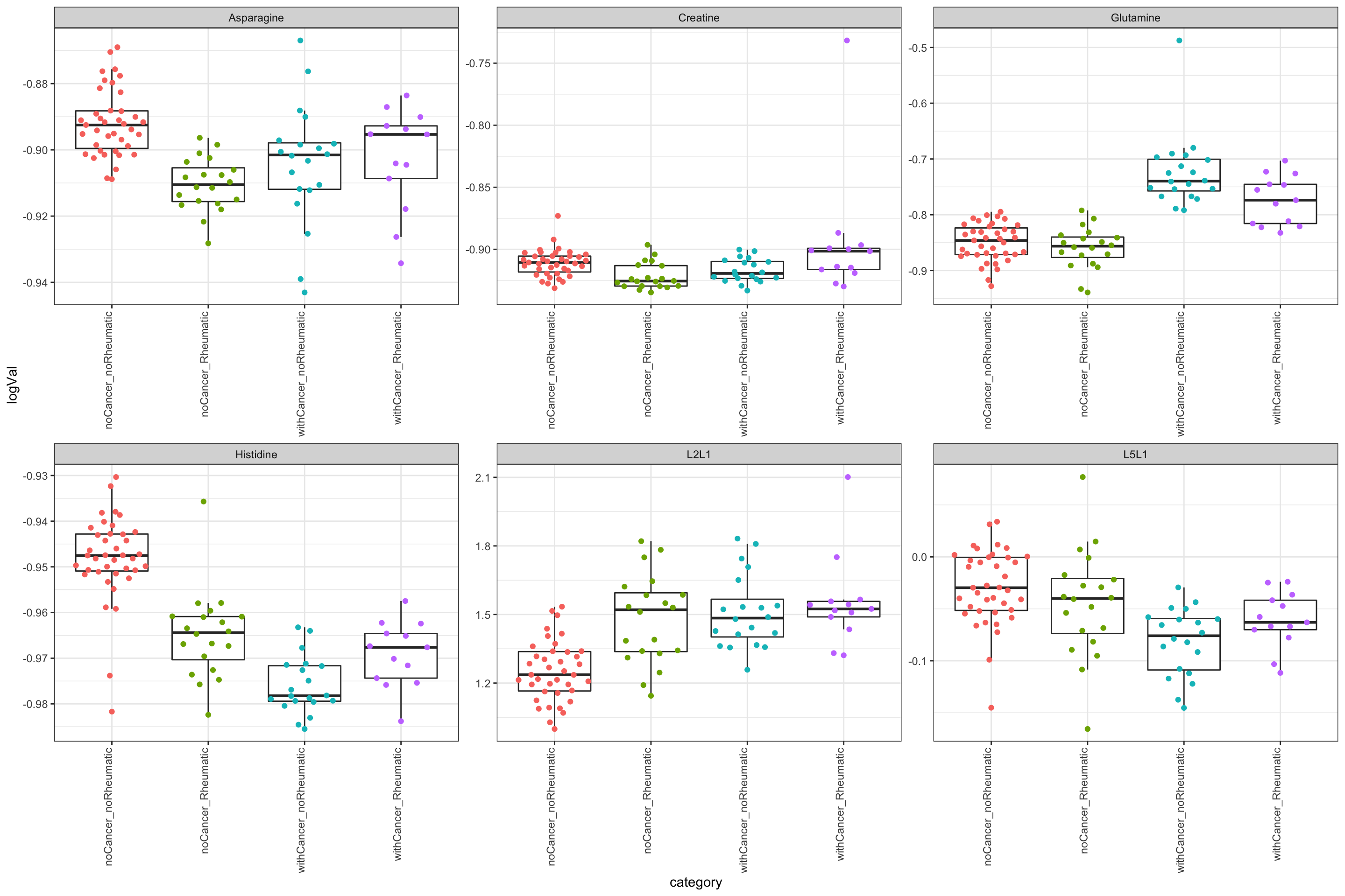

Different between cancer and non-cancer, regardless of irAE status

resTab.sig <- resTab %>% 
  filter(term == "cancer") %>%
  select(name, p.value) %>%
  arrange(p.value) %>%
  filter(p.value <= 0.05, !name %in% resTab.inter$name)
resTab.sig

# A tibble: 18 × 2
# Groups:   name [18]
   name             p.value
   <chr>              <dbl>
 1 Choline         9.26e-15
 2 L6L1            3.05e-13
 3 L3L1            6.89e-12
 4 Formate         2.10e-10
 5 Creatinine      1.62e- 9
 6 Aspartate       9.59e- 9
 7 Succinate       2.07e- 7
 8 Glucose         6.79e- 7
 9 Acetate         7.61e- 7
10 Glutamate       2.39e- 6
11 Hydroxybutyrate 2.59e- 5
12 L4L1            4.09e- 5
13 Isoleucine      8.67e- 5
14 Threonine       5.47e- 4
15 Tyrosine        3.63e- 3
16 Valine          4.44e- 3
17 Glycine         8.65e- 3
18 LysArg          2.06e- 2

Plot significant associations (p<=0.05)

plotTab <- filter(testTab, name %in% resTab.sig$name)
  
ggplot(plotTab, aes(x=cancer, y=logVal)) +
  geom_boxplot(outlier.shape = NA) +
  ggbeeswarm::geom_quasirandom(aes(col = cancer)) +
  theme_bw() +
  theme(plot.title = element_text(face="bold", hjust = 0.5),
        legend.position = "no",
        axis.text.x = element_text(angle = 90, hjust = 1, vjust = 0)) +
  facet_wrap(~name+irAE, scales = "free", ncol=4)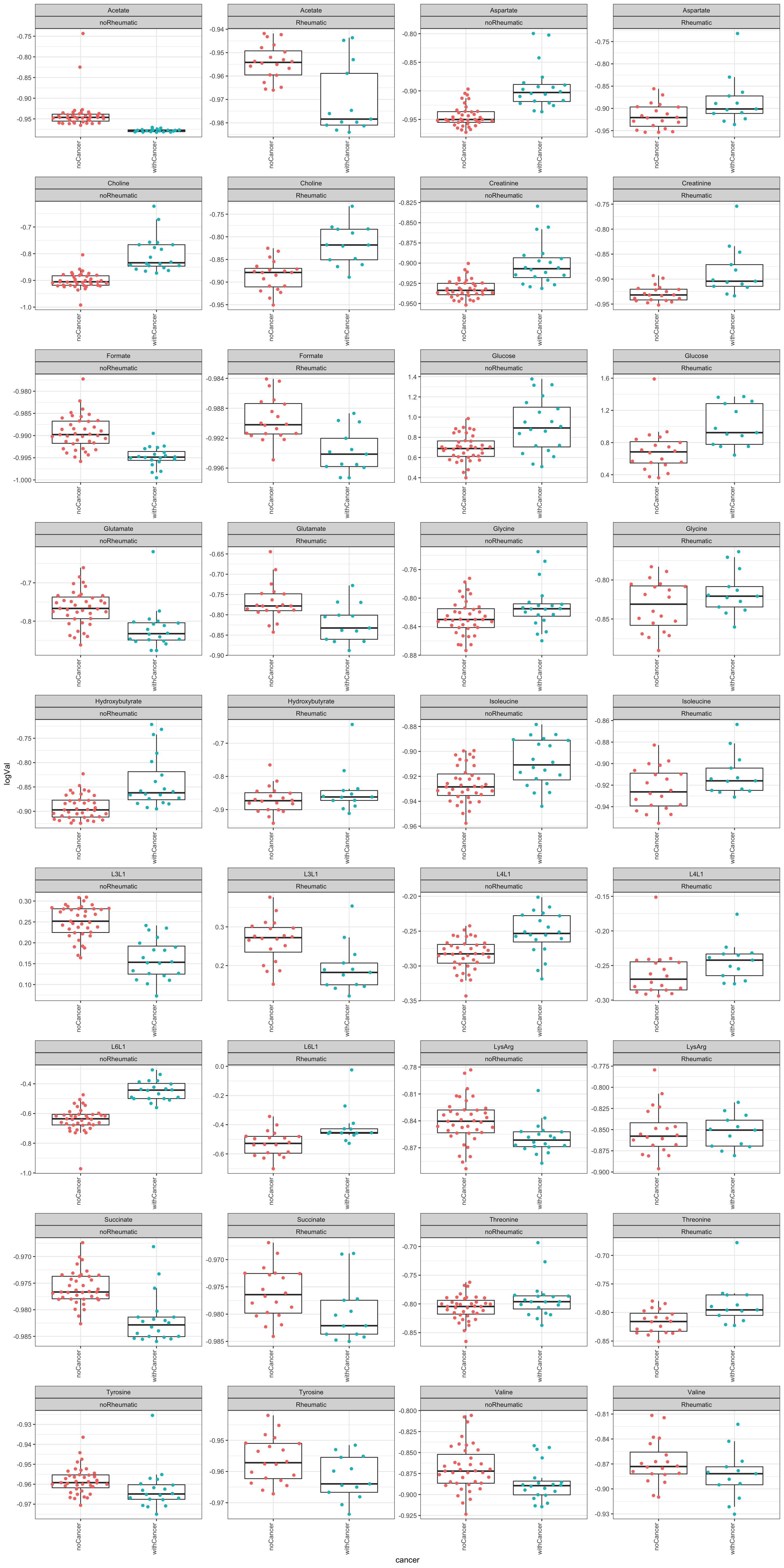

Different between irAE and no irAE, regardless of cancer

resTab.sig <- resTab %>% 
  filter(term == "irAE") %>%
  select(name, p.value) %>%
  arrange(p.value) %>%
  filter(p.value <= 0.05, !name %in% resTab.inter$name)
resTab.sig

# A tibble: 4 × 2
# Groups:   name [4]
  name        p.value
  <chr>         <dbl>
1 L6L1      0.0000419
2 Lactate   0.000267 
3 Aspartate 0.00431  
4 L4L1      0.00614

Plot significant associations (p<=0.05)

plotTab <- filter(testTab, name %in% resTab.sig$name)
  
ggplot(plotTab, aes(x=irAE, y=logVal)) +
  geom_boxplot(outlier.shape = NA) +
  ggbeeswarm::geom_quasirandom(aes(col = irAE)) +
  theme_bw() +
  theme(plot.title = element_text(face="bold", hjust = 0.5),
        legend.position = "no",
        axis.text.x = element_text(angle = 90, hjust = 1, vjust = 0)) +
  facet_wrap(~name+cancer, scales = "free", ncol=4)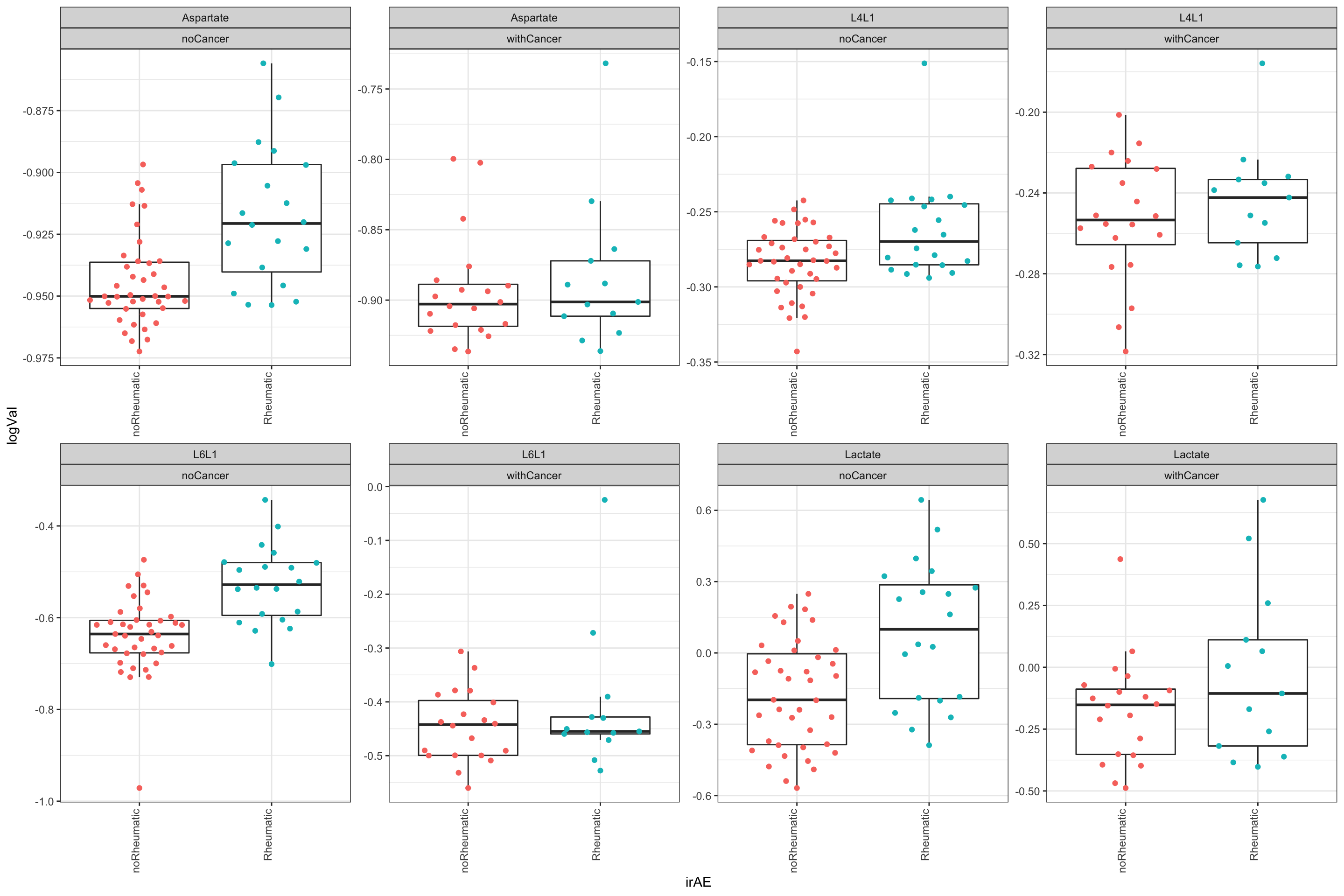

sessionInfo()

R version 4.2.0 (2022-04-22)
Platform: x86_64-apple-darwin17.0 (64-bit)
Running under: macOS Big Sur/Monterey 10.16

Matrix products: default
BLAS:   /Library/Frameworks/R.framework/Versions/4.2/Resources/lib/libRblas.0.dylib
LAPACK: /Library/Frameworks/R.framework/Versions/4.2/Resources/lib/libRlapack.dylib

locale:
[1] en_US.UTF-8/en_US.UTF-8/en_US.UTF-8/C/en_US.UTF-8/en_US.UTF-8

attached base packages:
[1] stats4    stats     graphics  grDevices utils     datasets  methods  
[8] base     

other attached packages:
 [1] forcats_0.5.1               stringr_1.4.0              
 [3] dplyr_1.0.9                 purrr_0.3.4                
 [5] readr_2.1.2                 tidyr_1.2.0                
 [7] tibble_3.1.8                ggplot2_3.3.6              
 [9] tidyverse_1.3.2             jyluMisc_0.1.5             
[11] vsn_3.64.0                  pheatmap_1.0.12            
[13] MultiAssayExperiment_1.22.0 SummarizedExperiment_1.26.1
[15] Biobase_2.56.0              GenomicRanges_1.48.0       
[17] GenomeInfoDb_1.32.2         IRanges_2.30.0             
[19] S4Vectors_0.34.0            BiocGenerics_0.42.0        
[21] MatrixGenerics_1.8.1        matrixStats_0.62.0         

loaded via a namespace (and not attached):
  [1] readxl_1.4.0           backports_1.4.1        fastmatch_1.1-3       
  [4] drc_3.0-1              workflowr_1.7.0        igraph_1.3.4          
  [7] shinydashboard_0.7.2   splines_4.2.0          BiocParallel_1.30.3   
 [10] TH.data_1.1-1          digest_0.6.29          htmltools_0.5.3       
 [13] fansi_1.0.3            magrittr_2.0.3         googlesheets4_1.0.0   
 [16] cluster_2.1.3          tzdb_0.3.0             limma_3.52.2          
 [19] modelr_0.1.8           sandwich_3.0-2         piano_2.12.0          
 [22] colorspace_2.0-3       rvest_1.0.2            haven_2.5.0           
 [25] xfun_0.31              crayon_1.5.1           RCurl_1.98-1.7        
 [28] jsonlite_1.8.0         survival_3.4-0         zoo_1.8-10            
 [31] glue_1.6.2             survminer_0.4.9        gtable_0.3.0          
 [34] gargle_1.2.0           zlibbioc_1.42.0        XVector_0.36.0        
 [37] DelayedArray_0.22.0    car_3.1-0              abind_1.4-5           
 [40] scales_1.2.0           mvtnorm_1.1-3          DBI_1.1.3             
 [43] relations_0.6-12       rstatix_0.7.0          Rcpp_1.0.9            
 [46] plotrix_3.8-2          xtable_1.8-4           preprocessCore_1.58.0 
 [49] km.ci_0.5-6            DT_0.23                httr_1.4.3            
 [52] htmlwidgets_1.5.4      fgsea_1.22.0           gplots_3.1.3          
 [55] RColorBrewer_1.1-3     ellipsis_0.3.2         farver_2.1.1          
 [58] pkgconfig_2.0.3        sass_0.4.2             dbplyr_2.2.1          
 [61] utf8_1.2.2             labeling_0.4.2         tidyselect_1.1.2      
 [64] rlang_1.0.4            later_1.3.0            munsell_0.5.0         
 [67] cellranger_1.1.0       tools_4.2.0            visNetwork_2.1.0      
 [70] cachem_1.0.6           cli_3.3.0              generics_0.1.3        
 [73] broom_1.0.0            evaluate_0.15          fastmap_1.1.0         
 [76] yaml_2.3.5             knitr_1.39             fs_1.5.2              
 [79] survMisc_0.5.6         caTools_1.18.2         mime_0.12             
 [82] slam_0.1-50            xml2_1.3.3             compiler_4.2.0        
 [85] rstudioapi_0.13        beeswarm_0.4.0         affyio_1.66.0         
 [88] ggsignif_0.6.3         marray_1.74.0          reprex_2.0.1          
 [91] bslib_0.4.0            stringi_1.7.8          highr_0.9             
 [94] lattice_0.20-45        Matrix_1.4-1           shinyjs_2.1.0         
 [97] KMsurv_0.1-5           vctrs_0.4.1            pillar_1.8.0          
[100] lifecycle_1.0.1        BiocManager_1.30.18    jquerylib_0.1.4       
[103] data.table_1.14.2      cowplot_1.1.1          bitops_1.0-7          
[106] httpuv_1.6.5           R6_2.5.1               affy_1.74.0           
[109] promises_1.2.0.1       KernSmooth_2.23-20     gridExtra_2.3         
[112] vipor_0.4.5            codetools_0.2-18       MASS_7.3-58           
[115] gtools_3.9.3           exactRankTests_0.8-35  assertthat_0.2.1      
[118] rprojroot_2.0.3        withr_2.5.0            multcomp_1.4-19       
[121] GenomeInfoDbData_1.2.8 parallel_4.2.0         hms_1.1.1             
[124] grid_4.2.0             rmarkdown_2.14         carData_3.0-5         
[127] googledrive_2.0.0      git2r_0.30.1           maxstat_0.7-25        
[130] ggpubr_0.4.0           sets_1.0-21            lubridate_1.8.0       
[133] shiny_1.7.2            ggbeeswarm_0.6.0

Perform association tests between molecular features and disease phenotypes for each dataset

Junyan Lu

Load packages

Analyses focused on cancer patients

CBA data

Baseline samples

PCA

Any PC separate different group?

ANOVA test

Pair-wise comparison between phenotypes

Follow-up samples

PCA

Any PC separate different group?

ANOVA

Pair-wise comparison

Use difference between follow_up and baseline

PCA

Any PC separate different group?

ANOVA

Pair-wise comparison

Summarise the pariwise comparison results using a heatmap

NMR data

Baseline samples

PCA

Any PC separate different group?

ANOVA

Pair-wise comparison

Follow-up samples

PCA

Any PC separate different group?

ANOVA

Pair-wise comparison

Use difference between follow_up and baseline

PCA

Any PC separate different group?

ANOVA

Pair-wise comparison

Summarise the pariwise comparison results using a heatmap

Focuse on cancer patients, combine rheumatic irAE and other irAE into one irAE group

CBA data

Baseline samples

PCA

Any PC separate different group?

ANOVA

Pair-wise comparison

Follow-up samples

PCA

Any PC separate different group?

ANOVA

Pair-wise comparison

Difference between follow_up and baseline

PCA

Any PC separate different group?

ANOVA

Pair-wise comparison

Summarise the pariwise comparison results using a heatmap

NMR data

Baseline samples

PCA

Any PC separate different group?

ANOVA

Pair-wise comparison

Follow-up samples

PCA

Any PC separate different group?

ANOVA

Pair-wise comparison

Use difference between follow_up and baseline

PCA

Any PC separate different group?

ANOVA

Pair-wise comparison

Summarise the pariwise comparison results using a heatmap

Analysis focused on none-cancer patients

CBA data

Baseline samples

PCA

Batch can be a confounder, remove sample with the second batch

Any PC separate different group?

ANOVA