Explore the CDK response signatures in CLL
Junyan Lu
17 May 2022
Last updated: 2022-05-17
Checks: 5 2
Knit directory: EMBL2016/analysis/
This reproducible R Markdown analysis was created with workflowr (version 1.7.0). The Checks tab describes the reproducibility checks that were applied when the results were created. The Past versions tab lists the development history.
The R Markdown is untracked by Git. To know which version of the R Markdown file created these results, you’ll want to first commit it to the Git repo. If you’re still working on the analysis, you can ignore this warning. When you’re finished, you can run wflow_publish to commit the R Markdown file and build the HTML.
Great job! The global environment was empty. Objects defined in the global environment can affect the analysis in your R Markdown file in unknown ways. For reproduciblity it’s best to always run the code in an empty environment.
The command set.seed(20210512) was run prior to running the code in the R Markdown file. Setting a seed ensures that any results that rely on randomness, e.g. subsampling or permutations, are reproducible.
Great job! Recording the operating system, R version, and package versions is critical for reproducibility.
- unnamed-chunk-27
To ensure reproducibility of the results, delete the cache directory CDK_analysis_cache and re-run the analysis. To have workflowr automatically delete the cache directory prior to building the file, set delete_cache = TRUE when running wflow_build() or wflow_publish().
Great job! Using relative paths to the files within your workflowr project makes it easier to run your code on other machines.
Great! You are using Git for version control. Tracking code development and connecting the code version to the results is critical for reproducibility.
The results in this page were generated with repository version 12d1722. See the Past versions tab to see a history of the changes made to the R Markdown and HTML files.
Note that you need to be careful to ensure that all relevant files for the analysis have been committed to Git prior to generating the results (you can use wflow_publish or wflow_git_commit). workflowr only checks the R Markdown file, but you know if there are other scripts or data files that it depends on. Below is the status of the Git repository when the results were generated:
Ignored files:
    Ignored:    .DS_Store
    Ignored:    .Rhistory
    Ignored:    analysis/.DS_Store
    Ignored:    analysis/.Rhistory
    Ignored:    analysis/CDK_analysis_cache/
    Ignored:    analysis/boxplot_AUC.png
    Ignored:    analysis/consensus_clustering_CPS_cache/
    Ignored:    analysis/consensus_clustering_noFit_cache/
    Ignored:    analysis/dose_curve.png
    Ignored:    analysis/targetDist.png
    Ignored:    analysis/toxivity_box.png
    Ignored:    analysis/volcano.png
    Ignored:    data/.DS_Store
    Ignored:    output/.DS_Store

Untracked files:
    Untracked:  analysis/AUC_CLL_IC50/
    Untracked:  analysis/BRAF_analysis.Rmd
    Untracked:  analysis/CDK_analysis.Rmd
    Untracked:  analysis/GSVA_analysis.Rmd
    Untracked:  analysis/NOTCH1_signature.Rmd
    Untracked:  analysis/autoluminescence.Rmd
    Untracked:  analysis/bar_plot_mixed.pdf
    Untracked:  analysis/bar_plot_mixed_noU1.pdf
    Untracked:  analysis/beatAML/
    Untracked:  analysis/cohortComposition_CLLsamples.pdf
    Untracked:  analysis/cohortComposition_allSamples.pdf
    Untracked:  analysis/consensus_clustering.Rmd
    Untracked:  analysis/consensus_clustering_CPS.Rmd
    Untracked:  analysis/consensus_clustering_IC50.Rmd
    Untracked:  analysis/consensus_clustering_beatAML.Rmd
    Untracked:  analysis/consensus_clustering_noFit.Rmd
    Untracked:  analysis/consensus_clusters.pdf
    Untracked:  analysis/disease_specific.Rmd
    Untracked:  analysis/dose_curve_selected.pdf
    Untracked:  analysis/genomic_association.Rmd
    Untracked:  analysis/genomic_association_allDisease.Rmd
    Untracked:  analysis/mean_autoluminescence_val.csv
    Untracked:  analysis/mean_autoluminescence_val.xlsx
    Untracked:  analysis/noFit_CLL/
    Untracked:  analysis/number_associations.pdf
    Untracked:  analysis/overview.Rmd
    Untracked:  analysis/plotCohort.Rmd
    Untracked:  analysis/preprocess.Rmd
    Untracked:  analysis/volcano_noBlocking.pdf
    Untracked:  code/utils.R
    Untracked:  data/BeatAML_Waves1_2/
    Untracked:  data/ic50Tab.RData
    Untracked:  data/newEMBL_20210806.RData
    Untracked:  data/patMeta.RData
    Untracked:  data/targetAnnotation_all.csv
    Untracked:  force_sync.sh
    Untracked:  output/gene_associations/
    Untracked:  output/resConsClust.RData
    Untracked:  output/resConsClust_aucFit.RData
    Untracked:  output/resConsClust_beatAML.RData
    Untracked:  output/resConsClust_cps.RData
    Untracked:  output/resConsClust_ic50.RData
    Untracked:  output/resConsClust_noFit.RData
    Untracked:  output/screenData.RData
    Untracked:  sync.sh

Unstaged changes:
    Modified:   _workflowr.yml
    Modified:   analysis/_site.yml
    Deleted:    analysis/about.Rmd
    Modified:   analysis/index.Rmd
    Deleted:    analysis/license.Rmd
Note that any generated files, e.g. HTML, png, CSS, etc., are not included in this status report because it is ok for generated content to have uncommitted changes.
There are no past versions. Publish this analysis with wflow_publish() to start tracking its development.
Load packages and datasets
library(jyluMisc)
library(tidyverse)

knitr::opts_chunk$set(warning = FALSE, message = FALSE)
#processed screen data
load("../output/screenData.RData")
#patient annotation
load("../data/patMeta.RData")Summarise the trend of CDKi responses
Choose the drugs selected by Jarno
drugList <- c("Dinaciclib", "THZ1", "SNS-032", "Flavopiridol", "AT7519", "R547","PHA-767491")
drugList
[1] "Dinaciclib" "THZ1" "SNS-032" "Flavopiridol" "AT7519"
[6] "R547" "PHA-767491" viabMat <- screenData %>% filter(diagnosis %in% "CLL", Drug %in% drugList) %>%
group_by(patientID, Drug) %>%
summarise(viab = mean(viab.auc)) %>%
pivot_wider(names_from = "patientID", values_from = "viab") %>%
column_to_rownames("Drug") %>% as.matrix()
patAnno <- patMeta %>% filter(Patient.ID %in% colnames(viabMat)) %>%
select(Patient.ID, IGHV.status, trisomy12, TP53, SF3B1, NOTCH1) %>%
dplyr::rename(patID = "Patient.ID")PCA
pcRes <- prcomp(t(viabMat), center = TRUE, scale. = TRUE)
pcTab <- pcRes$x[,1:2] %>% as_tibble(rownames = "patID") %>%
  left_join(patAnno)
varExp <- pcRes$sdev^2
varExp <- varExp/sum(varExp)
PCA plot
PCbiplot <- function(PC, x="PC1", y="PC2") {
# PC being a prcomp object
varExp = (pcRes$sdev^2)/sum(pcRes$sdev^2)
plotTab <- pcRes$x %>% data.frame() %>% rownames_to_column("patID") %>%
left_join(patAnno, by = "patID") %>%
filter(!is.na(IGHV.status),!is.na(trisomy12))
p <- ggplot(plotTab, aes(x=PC1, y=PC2)) +
geom_point(aes(color = IGHV.status, shape = trisomy12), size=3) +
theme_bw() + xlim(-5,5) + ylim(-5,5) +
xlab(sprintf("PC1 (%1.1f%%)", 100*varExp[1])) +
ylab(sprintf("PC2 (%1.1f%%)", 100*varExp[2])) +
theme(legend.position = "bottom")
datapc <- data.frame(varnames=rownames(PC$rotation), PC$rotation)
mult <- min(
(max(plotTab[,y]) - min(plotTab[,y])/(max(datapc[,y])-min(datapc[,y]))),
(max(plotTab[,x]) - min(plotTab[,x])/(max(datapc[,x])-min(datapc[,x])))
)
datapc <- transform(datapc,
v1 = .7 * mult * (get(x)),
v2 = .7 * mult * (get(y))
)
p <- p +
ggrepel::geom_text_repel(data=datapc, aes(x=v1, y=v2, label=varnames),
size = 5, vjust=1)
p <- p + geom_segment(data=datapc, aes(x=0, y=0, xend=v1, yend=v2), arrow=arrow(length=unit(0.2,"cm")), alpha=0.4)
p
}
PCbiplot(pcRes)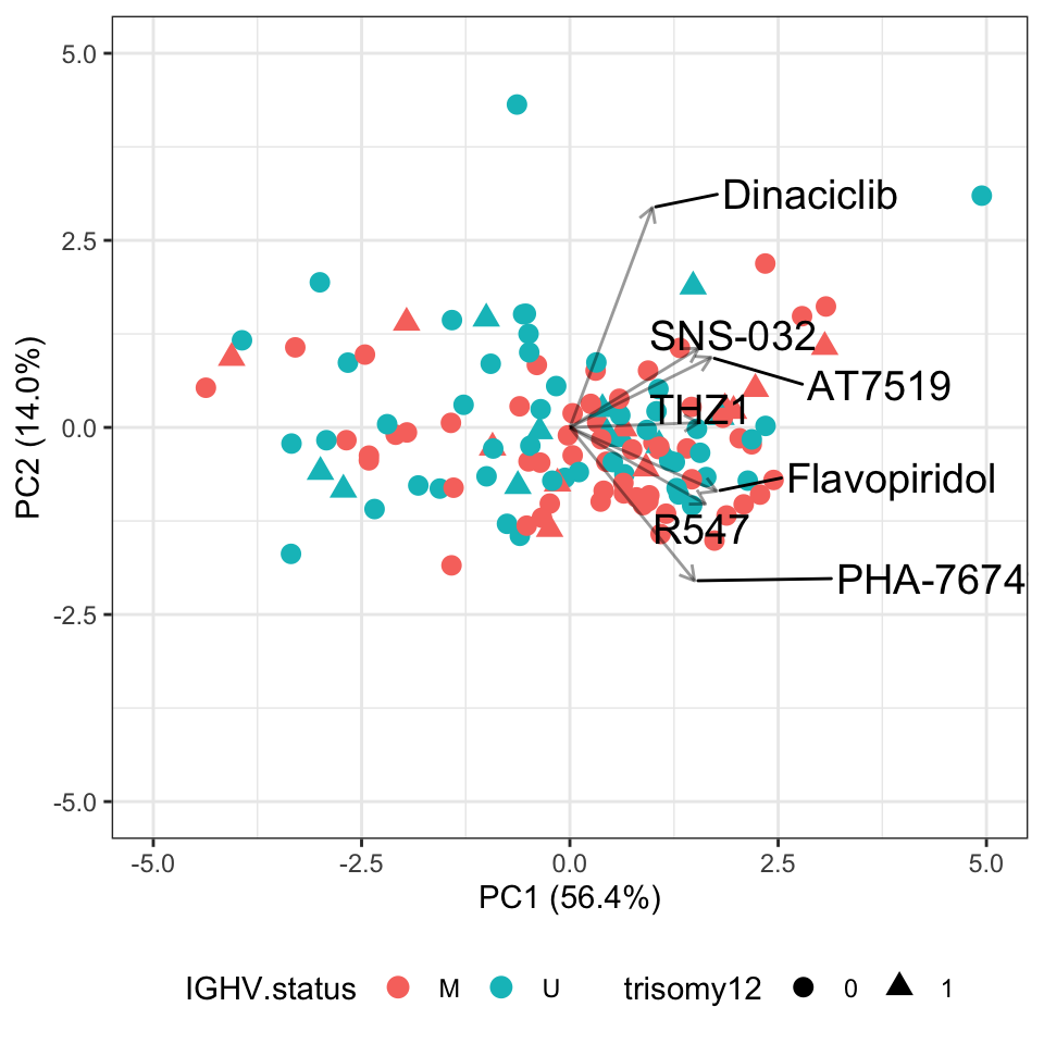 PC1 explains most of the variance, indicating those CDK inhibitors show similar trends. Perhaps except for Dinaciclib.
Heatmap of viabilities, ordered by PC1 value (not scaled)
library(pheatmap)
viabMat <- viabMat[,arrange(pcTab, PC1)$patID]
colAnno <- patAnno %>% mutate(PC1 = pcTab[match(patID, pcTab$patID),]$PC1) %>%
  column_to_rownames("patID") %>% data.frame()

pheatmap(viabMat, cluster_cols = FALSE, cluster_rows = TRUE, annotation_col = colAnno, scale = "none")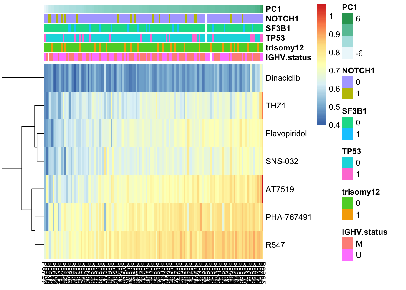
Heatmap of viabilities, ordered by PC1 value (row-scaled)
library(pheatmap)
pheatmap(viabMat, cluster_cols = FALSE, cluster_rows = TRUE, annotation_col = colAnno, scale = "row")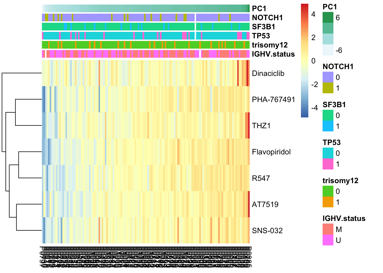 Higher PC1 is associated with more resistant to CDK inhibitors
Correlation plot
library(corrplot)
corrplot(cor(t(viabMat)))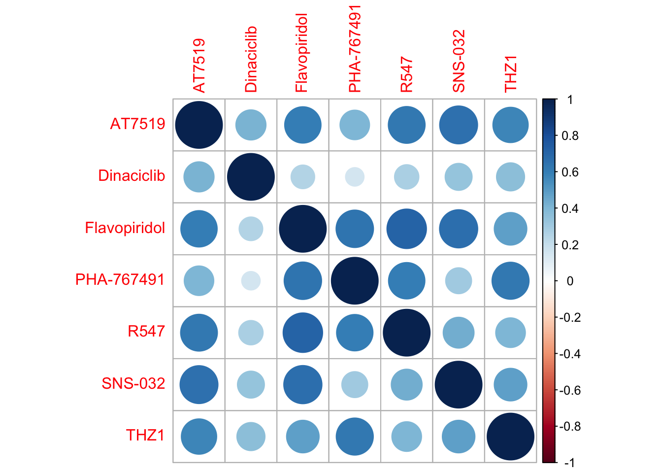
We can use PC1 to summarise the general gradient of the response to CDK inhibitors, as the response patterns of those inhibitors are quite similar.
Associations with genomics
Prepare genomic data
geneTab <- patMeta %>% select(Patient.ID, IGHV.status, del10p:U1) %>%
  filter(Patient.ID %in% pcTab$patID) %>%
  mutate(IGHV.status = as.factor(2-as.numeric(as.factor(IGHV.status)))) %>%
  pivot_longer(-Patient.ID)

sumTab <- group_by(geneTab, name) %>%
  summarise(fracNA = sum(is.na(value))/length(pcTab$patID),
            numMut = sum(value %in% 1)) %>%
  filter(numMut >=3, fracNA <= 0.2)
geneTab <- filter(geneTab, name %in% sumTab$name)
Perform t-test
testTab <- pcTab %>% select(patID, PC1) %>%
  full_join(geneTab, by = c(patID = "Patient.ID"))

resTab <- group_by(testTab, name) %>% nest() %>%
  mutate(m=map(data, ~t.test(PC1 ~ value,., var.equal=TRUE))) %>%
  mutate(res = map(m, broom::tidy)) %>%
  unnest(res) %>%
  select(name, p.value, estimate) %>%
  arrange(p.value)
head(resTab)
# A tibble: 6 × 3
# Groups: name [6]
name p.value estimate
<chr> <dbl> <dbl>
1 del17p 0.0452 1.20
2 del9q 0.0497 -1.77
3 BRAF 0.0557 1.59
4 FAT4 0.0710 -1.51
5 NOTCH1 0.0935 0.869
6 EGR2 0.114 -1.23 Boxplots
pList <- lapply(filter(resTab,p.value < 0.05)$name, function(x) {
plotTab <- filter(testTab, name == x)
ggplot(plotTab, aes(x=value, y=PC1, col=factor(value))) +
geom_boxplot() + ggbeeswarm::geom_quasirandom() +
theme(legend.position = "none") +
ggtitle(x)
})
cowplot::plot_grid(plotlist = pList, ncol=2)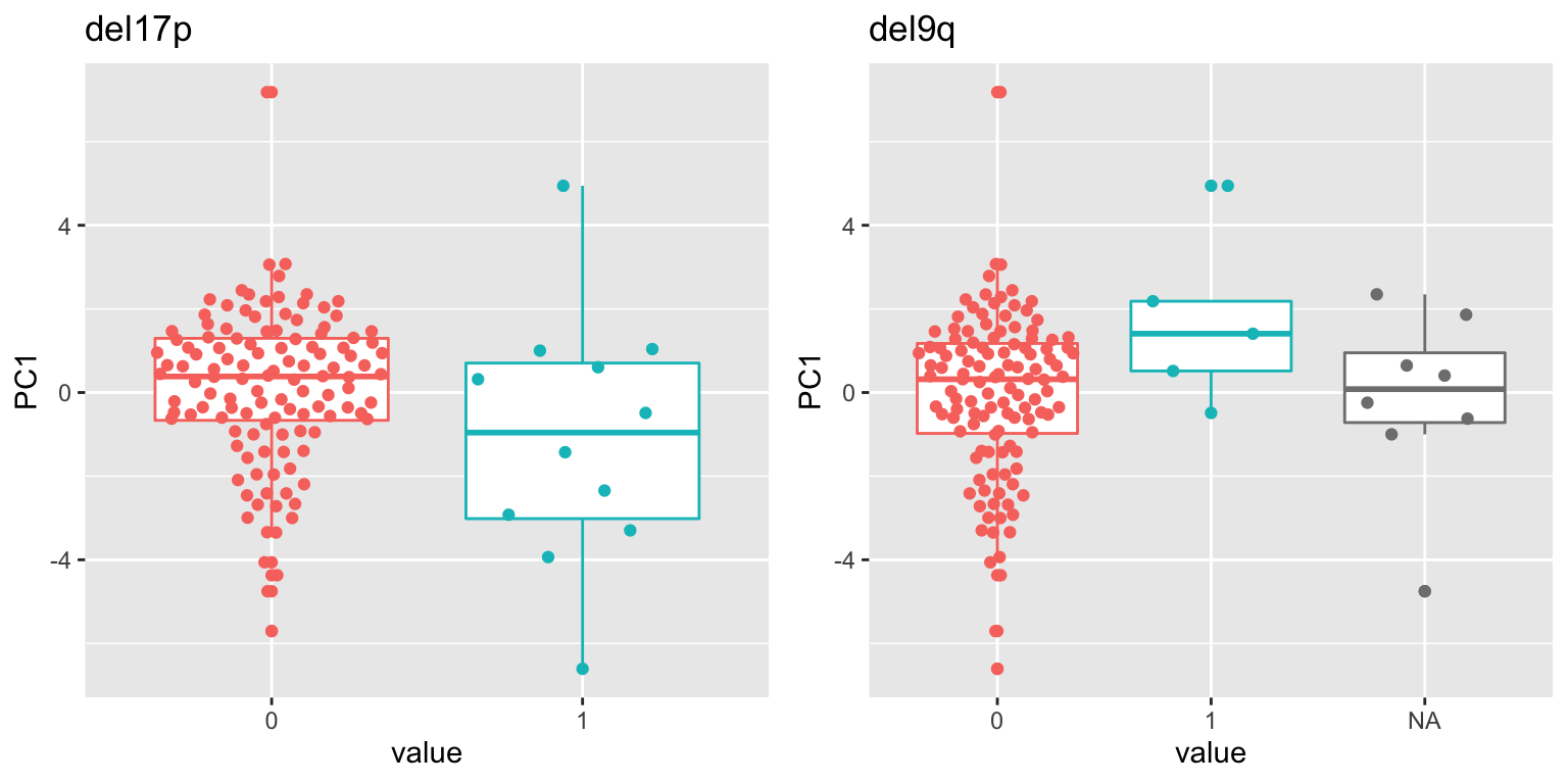 del17p shows some weak association. # Association with mRNA expression
Pre-processing
Subsetting
load("~/CLLproject_jlu/var/ddsrna_180717.RData")
ddsSub <- dds[,dds$PatID %in% pcTab$patID]
ddsSub$PC1 <- pcTab[match(ddsSub$PatID, pcTab$patID),]$PC1
ddsSub$IGHV <- patMeta[match(ddsSub$PatID, patMeta$Patient.ID),]$IGHV.status
ddsSub$trisomy12 <- patMeta[match(ddsSub$PatID, patMeta$Patient.ID),]$trisomy12
ddsSub <- ddsSub[,!is.na(ddsSub$IGHV) & !is.na(ddsSub$trisomy12)]
#remove low abundance genes
ddsSub <- ddsSub[rowMedians(counts(ddsSub, normalized = TRUE),na.rm = TRUE)>10,]
#keep protein coding genes
ddsSub <- ddsSub[rowData(ddsSub)$biotype %in% "protein_coding" & !rowData(ddsSub)$symbol %in% c(NA,""),]
Voom transformation
countMat <- counts(ddsSub)
exprMat <- limma::voom(counts = countMat, lib.size = ddsSub$sizeFactor)$E
Remove invariant genes
sds <- genefilter::rowSds(exprMat)
exprMat <- exprMat[sds > genefilter::shorth(sds),]
Correlation test using Limma
library(limma)
designMat <- model.matrix(~PC1+IGHV+trisomy12, colData(ddsSub))
fit <- lmFit(exprMat, designMat)
fit2 <- eBayes(fit)
resTab <- topTable(fit2, coef = "PC1", number =Inf) %>%
  as_tibble(rownames ="id") %>%
  mutate(symbol = rowData(ddsSub)[id,]$symbol)
P-value histogram
hist(resTab$P.Value)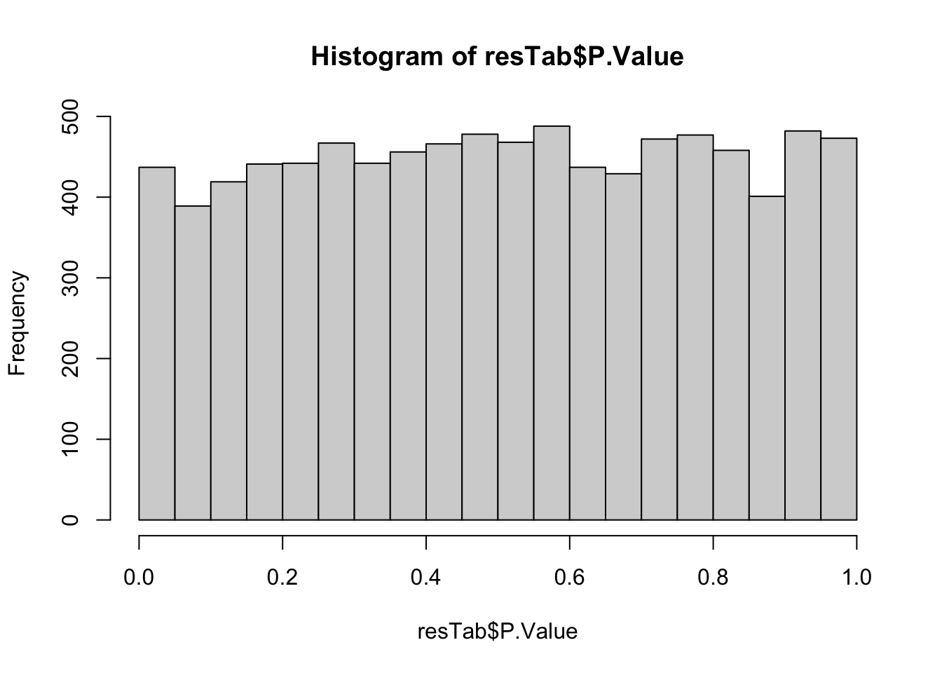 Associations are not strong.
Genes passed raw p value < 0.05 (none association passed 10% FDR)
resTab.sig <- filter(resTab, P.Value < 0.05)
resTab.sig %>% mutate_if(is.numeric, formatC, digits=2) %>%
  DT::datatable()
Boxplot of top9 genes
pList <- lapply(seq(9), function(i) {
rec <- resTab.sig[i,]
plotTab <- tibble(expr = exprMat[rec$id,],
PC1 = designMat[,"PC1"],
IGHV=factor(designMat[,"IGHVU"]))
ggplot(plotTab, aes(x=PC1, y=expr)) +
geom_point(aes(col = IGHV)) + geom_smooth(method = "lm") +
ggtitle(sprintf("%s (p=%s)",rec$symbol, formatC(rec$P.Value, digits=2)))
})
cowplot::plot_grid(plotlist= pList, ncol=3)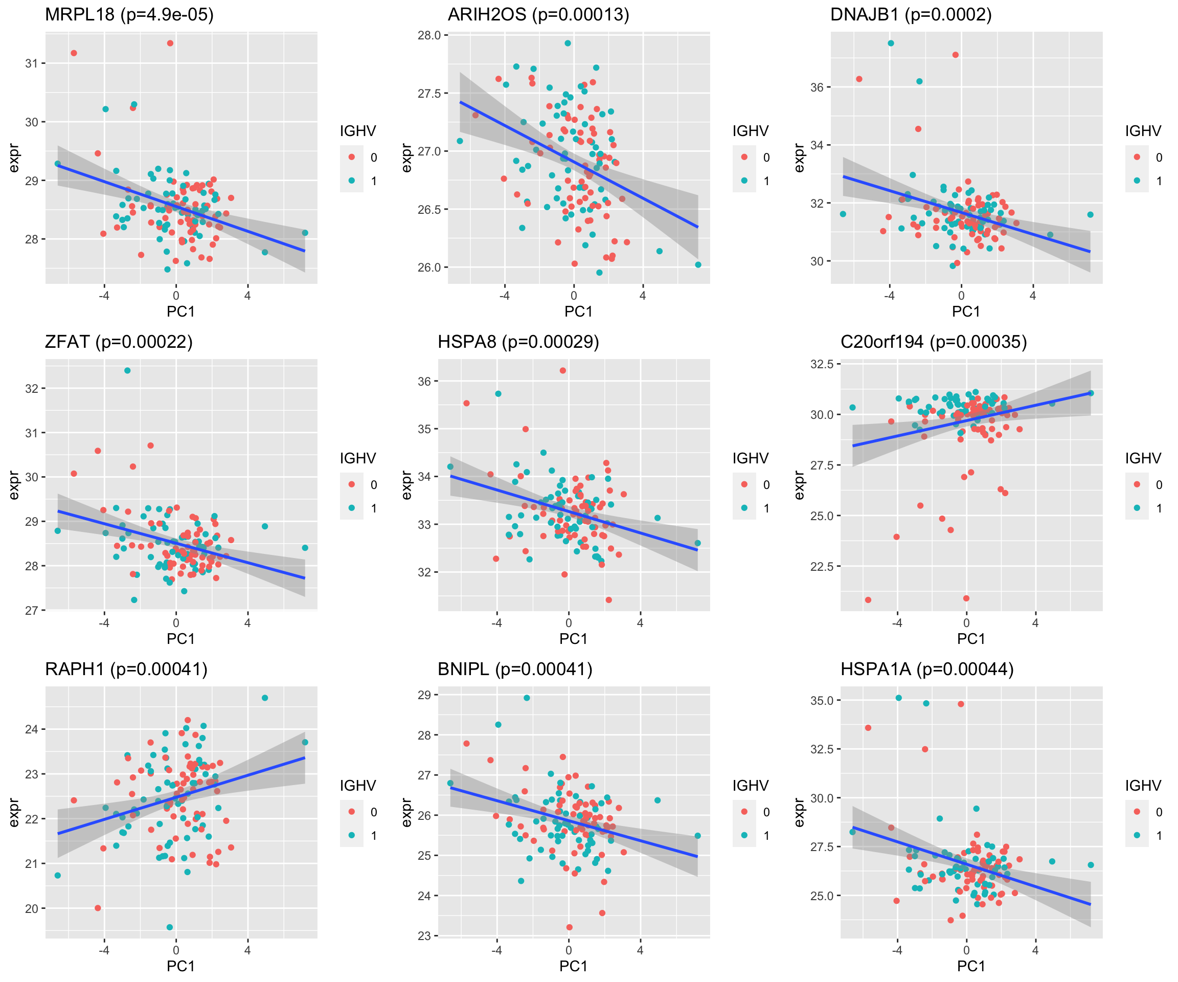 According the scatter plot, the associations are very moderate even though they passed 0.05 p-value
Pathway enrichment analysis
gmts <- list(H = "~/CLLproject_jlu/data/commonFiles/h.all.v6.2.symbols.gmt",
             KEGG = "~/CLLproject_jlu/data/commonFiles/c2.cp.kegg.v6.2.symbols.gmt",
             C6 = "~/CLLproject_jlu/data/commonFiles/c6.all.v6.2.symbols.gmt")
Cancer hallmmarks
resEnrich <- runCamera(exprMat, designMat, gmts$H, id = rowData(ddsSub)$symbol, pCut = 0.1, ifFDR = TRUE)[1] "No sets passed the criteria"resEnrich$enrichPlotNULLKEGG
resEnrich <- runCamera(exprMat, designMat, gmts$KEGG, id = rowData(ddsSub)$symbol, pCut = 0.1, ifFDR = TRUE)[1] "No sets passed the criteria"resEnrich$enrichPlotNULLOncogenetic
resEnrich <- runCamera(exprMat, designMat, gmts$C6, id = rowData(ddsSub)$symbol, pCut = 0.1, ifFDR = TRUE)[1] "No sets passed the criteria"resEnrich$enrichPlotNULLAssociation with protein expression
Load datasets
library(proDA)
library(SummarizedExperiment)

#load datasets
load("~/CLLproject_jlu/var/proteomic_LUMOS_batch13.RData")
Preprocessing
protCLL$PC1 <- pcTab[match(colnames(protCLL), pcTab$patID),]$PC1
protCLL <- protCLL[,!is.na(protCLL$IGHV.status) & !is.na(protCLL$trisomy12) & !is.na(protCLL$PC1)]
protMat <- assays(protCLL)[["count"]] #without imputation
protMatLog <- assays(protCLL)[["log2Norm"]]
Sample size
dim(protCLL)[1] 3314 56Differential expression
colData <- data.frame(colData(protCLL))[,c("batch","IGHV.status","trisomy12","PC1")]
fit <- proDA(protMat, design = ~ . ,  col_data =  colData)
resTab <- test_diff(fit, "PC1") %>%
dplyr::rename(id = name, logFC = diff, t=t_statistic,
P.Value = pval, adj.P.Val = adj_pval) %>%
mutate(name = rowData(protCLL[id,])$hgnc_symbol) %>%
select(name, id, logFC, t, P.Value, adj.P.Val, n_obs) %>%
arrange(P.Value) %>%
as_tibble()hist(resTab$P.Value)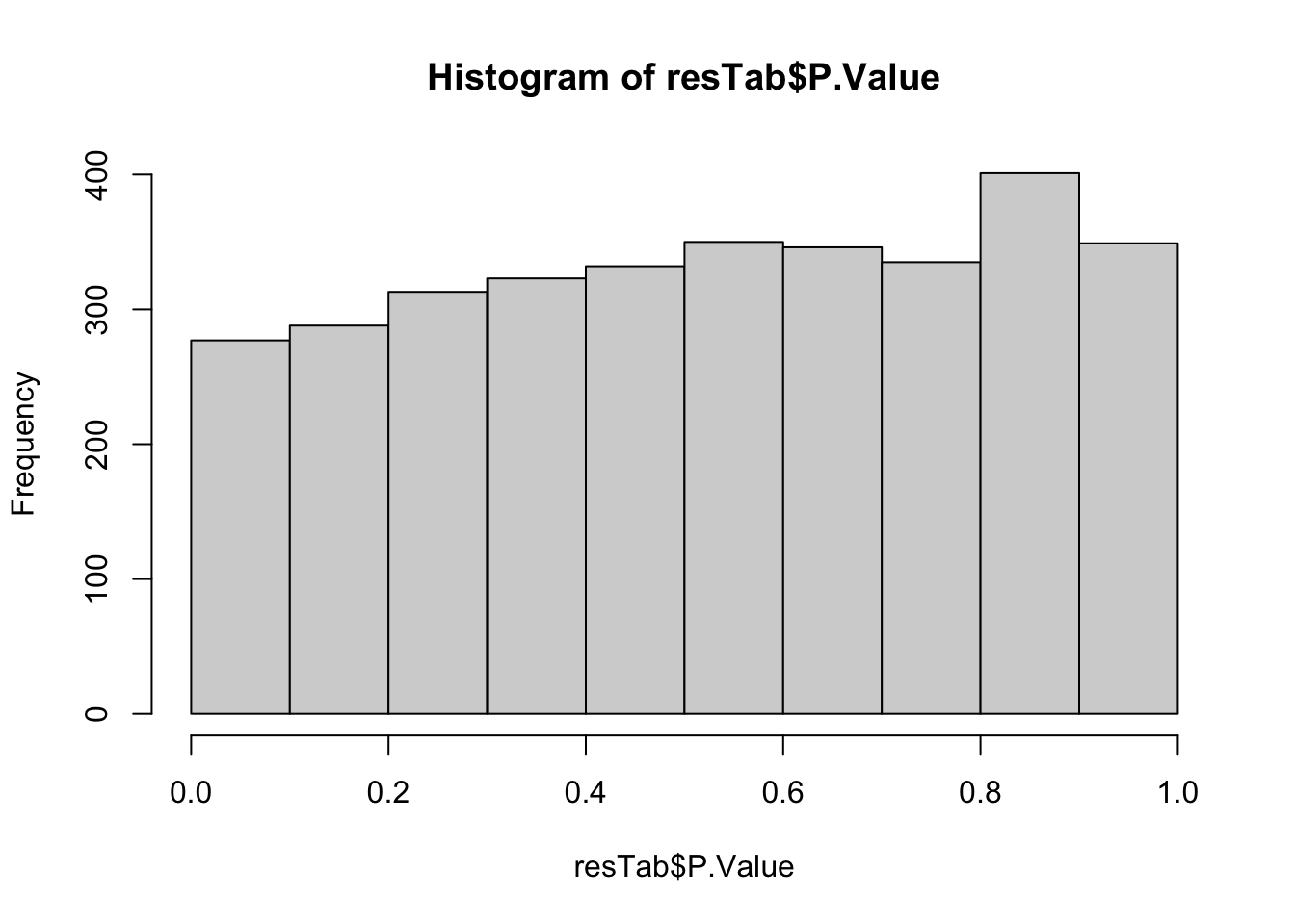 No clear associations
Table of proteins with raw p-values <0.05 (no results passed 10% FDR)
resTab.sig <- filter(resTab, P.Value < 0.05)
resTab.sig %>%
  mutate_if(is.numeric, formatC, digits=2) %>%
  DT::datatable()
Boxplot of top9 associations
pList <- lapply(seq(9), function(i) {
  rec <- resTab.sig[i,]
  plotTab <- tibble(expr = protMat[rec$id,],
                    PC1 = colData[,"PC1"],
                    IGHV=factor(colData[,"IGHV.status"]))
  ggplot(plotTab, aes(x=PC1, y=expr)) +
    geom_point(aes(col = IGHV)) + geom_smooth(method = "lm") +
    ggtitle(sprintf("%s (p=%s)",rec$name, formatC(rec$P.Value, digits=2)))
})
cowplot::plot_grid(plotlist= pList, ncol=3)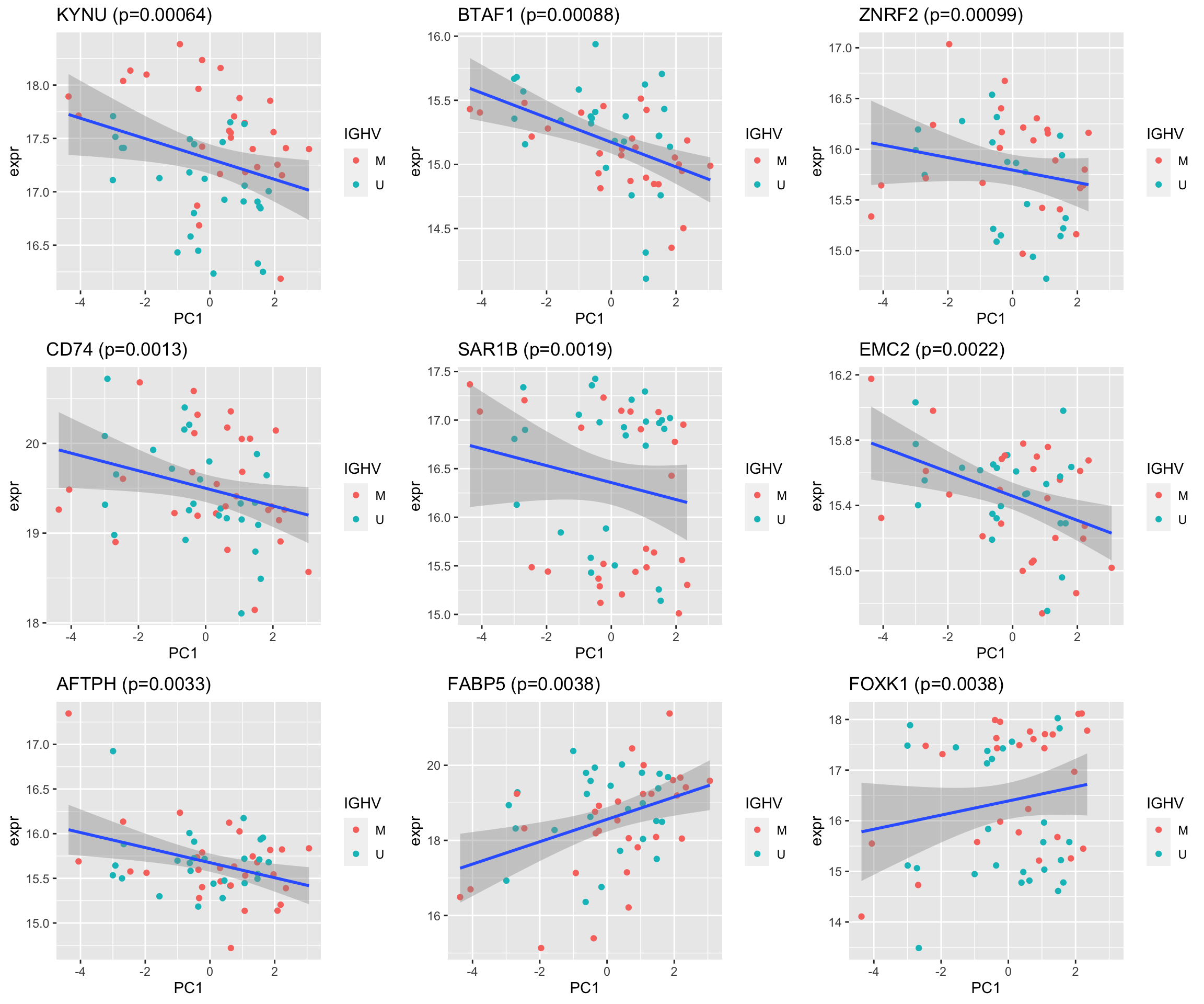
Pathway enrichment analysis
designMat <- model.matrix(~ batch + IGHV.status+trisomy12+PC1, colData)Cancer hallmmarks
protImp <- assays(protCLL)[["QRILC"]]
resEnrich <- runCamera(protImp, designMat, gmts$H, id = rowData(protCLL)$hgnc_symbol, pCut = 0.1, ifFDR = TRUE, contrast = "PC1")
[1] "No sets passed the criteria"KEGG
resEnrich <- runCamera(protImp, designMat, gmts$KEGG, id = rowData(protCLL)$hgnc_symbol, pCut = 0.1, ifFDR = TRUE, contrast = "PC1")
resEnrich$enrichPlot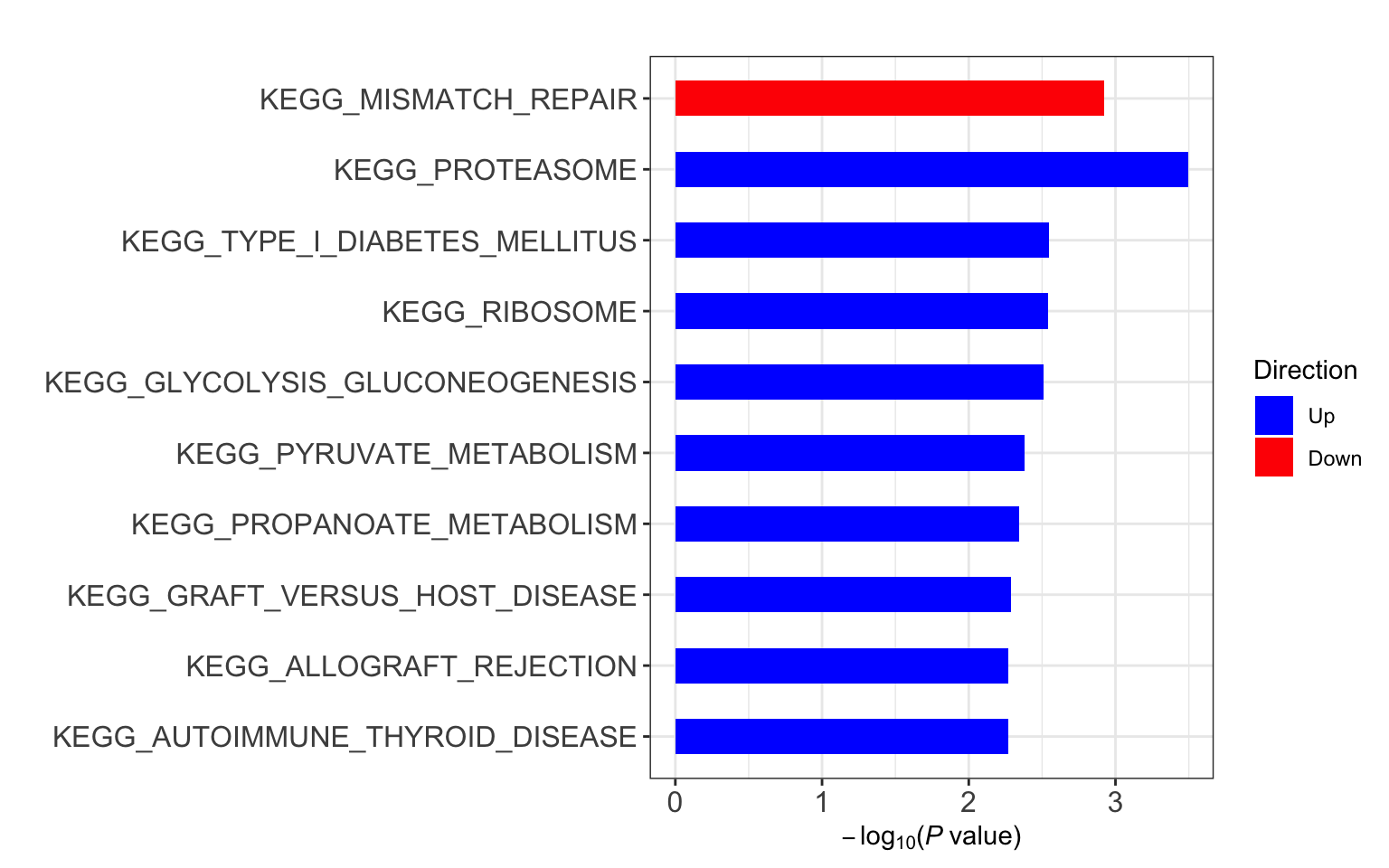
Oncogenetic
resEnrich <- runCamera(protImp, designMat, gmts$C6, id = rowData(protCLL)$hgnc_symbol, pCut = 0.1, ifFDR = TRUE,contrast = "PC1")[1] "No sets passed the criteria"resEnrich$enrichPlotNULLAssociations with BH3 profiling
BH3 profiling measures the cytochrome C release after treatment of BH3 peptides, to evaluate the sensitivity of cells to pro-apoptotic signals.
Preprocessing
load("../../BH3profiling/output/dynamicBH3.RData")
bh3Tab <- dynamicBH3 %>% filter(drug == "DMSO") %>%
  group_by(patID, peptide) %>%
  summarise(auc = mean(AUC))
Association test
testTab <- pcTab %>% full_join(bh3Tab, by = "patID") %>%
  filter(!is.na(auc),!is.na(PC1))
resTab <- group_by(testTab, peptide) %>% nest() %>%
  mutate(m = map(data, ~cor.test(~PC1+auc,.))) %>%
  mutate(res = map(m, broom::tidy)) %>%
  unnest(res) %>% arrange(p.value) %>%
  ungroup() %>%
  select(peptide, estimate, p.value) %>%
  mutate(p.adj = p.adjust(p.value, method= "BH"))
Result table
resTab %>% mutate_if(is.numeric, formatC, digits=2) %>% DT::datatable()Plot significant associations (p<0.05)
pList <- lapply(filter(resTab,p.value < 0.05)$peptide, function(x) {
  plotTab <- filter(testTab, peptide == x)
  ggplot(plotTab, aes(x=auc, y=PC1)) +
    geom_point(aes(col=IGHV.status)) + geom_smooth(method ="lm") +
    ggtitle(x) +
    xlab("BH3 priming")
})
cowplot::plot_grid(plotlist = pList, ncol=2)
Associations are pretty weak.
sessionInfo()R version 4.2.0 (2022-04-22)
Platform: x86_64-apple-darwin17.0 (64-bit)
Running under: macOS Big Sur/Monterey 10.16
Matrix products: default
BLAS: /Library/Frameworks/R.framework/Versions/4.2/Resources/lib/libRblas.0.dylib
LAPACK: /Library/Frameworks/R.framework/Versions/4.2/Resources/lib/libRlapack.dylib
locale:
[1] en_US.UTF-8/en_US.UTF-8/en_US.UTF-8/C/en_US.UTF-8/en_US.UTF-8
attached base packages:
[1] stats4 stats graphics grDevices utils datasets methods
[8] base
other attached packages:
[1] proDA_1.10.0 limma_3.52.0
[3] DESeq2_1.36.0 SummarizedExperiment_1.26.1
[5] Biobase_2.56.0 MatrixGenerics_1.8.0
[7] matrixStats_0.62.0 GenomicRanges_1.48.0
[9] GenomeInfoDb_1.32.1 IRanges_2.30.0
[11] S4Vectors_0.34.0 BiocGenerics_0.42.0
[13] corrplot_0.92 pheatmap_1.0.12
[15] forcats_0.5.1 stringr_1.4.0
[17] dplyr_1.0.9 purrr_0.3.4
[19] readr_2.1.2 tidyr_1.2.0
[21] tibble_3.1.7 ggplot2_3.3.6
[23] tidyverse_1.3.1 jyluMisc_0.1.5
loaded via a namespace (and not attached):
[1] utf8_1.2.2 shinydashboard_0.7.2 tidyselect_1.1.2
[4] RSQLite_2.2.14 AnnotationDbi_1.58.0 htmlwidgets_1.5.4
[7] grid_4.2.0 BiocParallel_1.30.0 maxstat_0.7-25
[10] munsell_0.5.0 codetools_0.2-18 DT_0.23
[13] withr_2.5.0 colorspace_2.0-3 highr_0.9
[16] knitr_1.39 rstudioapi_0.13 ggsignif_0.6.3
[19] labeling_0.4.2 git2r_0.30.1 slam_0.1-50
[22] GenomeInfoDbData_1.2.8 KMsurv_0.1-5 bit64_4.0.5
[25] farver_2.1.0 rprojroot_2.0.3 vctrs_0.4.1
[28] generics_0.1.2 TH.data_1.1-1 xfun_0.31
[31] sets_1.0-21 R6_2.5.1 ggbeeswarm_0.6.0
[34] locfit_1.5-9.5 bitops_1.0-7 cachem_1.0.6
[37] fgsea_1.22.0 DelayedArray_0.22.0 assertthat_0.2.1
[40] promises_1.2.0.1 scales_1.2.0 multcomp_1.4-19
[43] beeswarm_0.4.0 gtable_0.3.0 sandwich_3.0-1
[46] workflowr_1.7.0 rlang_1.0.2 genefilter_1.78.0
[49] splines_4.2.0 rstatix_0.7.0 broom_0.8.0
[52] BiocManager_1.30.17 yaml_2.3.5 abind_1.4-5
[55] modelr_0.1.8 crosstalk_1.2.0 backports_1.4.1
[58] httpuv_1.6.5 tools_4.2.0 relations_0.6-12
[61] ellipsis_0.3.2 gplots_3.1.3 jquerylib_0.1.4
[64] RColorBrewer_1.1-3 Rcpp_1.0.8.3 visNetwork_2.1.0
[67] zlibbioc_1.42.0 RCurl_1.98-1.6 ggpubr_0.4.0
[70] cowplot_1.1.1 zoo_1.8-10 haven_2.5.0
[73] ggrepel_0.9.1 cluster_2.1.3 exactRankTests_0.8-35
[76] fs_1.5.2 magrittr_2.0.3 data.table_1.14.2
[79] reprex_2.0.1 survminer_0.4.9 mvtnorm_1.1-3
[82] hms_1.1.1 shinyjs_2.1.0 mime_0.12
[85] evaluate_0.15 xtable_1.8-4 XML_3.99-0.9
[88] readxl_1.4.0 gridExtra_2.3 compiler_4.2.0
[91] KernSmooth_2.23-20 crayon_1.5.1 htmltools_0.5.2
[94] mgcv_1.8-40 later_1.3.0 tzdb_0.3.0
[97] geneplotter_1.74.0 lubridate_1.8.0 DBI_1.1.2
[100] dbplyr_2.1.1 MASS_7.3-57 BiocStyle_2.24.0
[103] Matrix_1.4-1 car_3.0-13 cli_3.3.0
[106] marray_1.74.0 parallel_4.2.0 igraph_1.3.1
[109] pkgconfig_2.0.3 km.ci_0.5-6 piano_2.12.0
[112] xml2_1.3.3 annotate_1.74.0 vipor_0.4.5
[115] bslib_0.3.1 XVector_0.36.0 drc_3.0-1
[118] rvest_1.0.2 digest_0.6.29 Biostrings_2.64.0
[121] rmarkdown_2.14 cellranger_1.1.0 fastmatch_1.1-3
[124] survMisc_0.5.6 shiny_1.7.1 gtools_3.9.2
[127] nlme_3.1-157 lifecycle_1.0.1 jsonlite_1.8.0
[130] carData_3.0-5 fansi_1.0.3 pillar_1.7.0
[133] lattice_0.20-45 KEGGREST_1.36.0 fastmap_1.1.0
[136] httr_1.4.3 plotrix_3.8-2 survival_3.3-1
[139] glue_1.6.2 png_0.1-7 bit_4.0.4
[142] stringi_1.7.6 sass_0.4.1 blob_1.2.3
[145] caTools_1.18.2 memoise_2.0.1