MOFA analysis for EMBL screen data
Junyan Lu
Last updated: 2022-07-12
Checks: 6 1
Knit directory: EMBL2016/analysis/
This reproducible R Markdown analysis was created with workflowr (version 1.7.0). The Checks tab describes the reproducibility checks that were applied when the results were created. The Past versions tab lists the development history.
The R Markdown is untracked by Git. To know which version of the R
Markdown file created these results, you’ll want to first commit it to
the Git repo. If you’re still working on the analysis, you can ignore
this warning. When you’re finished, you can run
wflow_publish to commit the R Markdown file and build the
HTML.
Great job! The global environment was empty. Objects defined in the global environment can affect the analysis in your R Markdown file in unknown ways. For reproduciblity it’s best to always run the code in an empty environment.
The command set.seed(20210512) was run prior to running
the code in the R Markdown file. Setting a seed ensures that any results
that rely on randomness, e.g. subsampling or permutations, are
reproducible.
Great job! Recording the operating system, R version, and package versions is critical for reproducibility.
Nice! There were no cached chunks for this analysis, so you can be confident that you successfully produced the results during this run.
Great job! Using relative paths to the files within your workflowr project makes it easier to run your code on other machines.
Great! You are using Git for version control. Tracking code development and connecting the code version to the results is critical for reproducibility.
The results in this page were generated with repository version 12d1722. See the Past versions tab to see a history of the changes made to the R Markdown and HTML files.
Note that you need to be careful to ensure that all relevant files for
the analysis have been committed to Git prior to generating the results
(you can use wflow_publish or
wflow_git_commit). workflowr only checks the R Markdown
file, but you know if there are other scripts or data files that it
depends on. Below is the status of the Git repository when the results
were generated:
Ignored files:
    Ignored:    .DS_Store
    Ignored:    .Rhistory
    Ignored:    analysis/.DS_Store
    Ignored:    analysis/.RData
    Ignored:    analysis/.Rhistory
    Ignored:    analysis/CDK_analysis_cache/
    Ignored:    analysis/boxplot_AUC.png
    Ignored:    analysis/consensus_clustering_CPS_cache/
    Ignored:    analysis/consensus_clustering_noFit_cache/
    Ignored:    analysis/dose_curve.png
    Ignored:    analysis/targetDist.png
    Ignored:    analysis/toxivity_box.png
    Ignored:    analysis/volcano.png
    Ignored:    data/.DS_Store
    Ignored:    output/.DS_Store

Untracked files:
    Untracked:  analysis/AUC_CLL_IC50/
    Untracked:  analysis/BRAF_analysis.Rmd
    Untracked:  analysis/CDK_analysis.Rmd
    Untracked:  analysis/GSVA_analysis.Rmd
    Untracked:  analysis/MOFA_analysis.Rmd
    Untracked:  analysis/NOTCH1_signature.Rmd
    Untracked:  analysis/autoluminescence.Rmd
    Untracked:  analysis/bar_plot_mixed.pdf
    Untracked:  analysis/bar_plot_mixed_noU1.pdf
    Untracked:  analysis/beatAML/
    Untracked:  analysis/cohortComposition_CLLsamples.pdf
    Untracked:  analysis/cohortComposition_allSamples.pdf
    Untracked:  analysis/consensus_clustering.Rmd
    Untracked:  analysis/consensus_clustering_CPS.Rmd
    Untracked:  analysis/consensus_clustering_IC50.Rmd
    Untracked:  analysis/consensus_clustering_beatAML.Rmd
    Untracked:  analysis/consensus_clustering_noFit.Rmd
    Untracked:  analysis/consensus_clusters.pdf
    Untracked:  analysis/coxResTab.RData
    Untracked:  analysis/disease_specific.Rmd
    Untracked:  analysis/dose_curve_selected.pdf
    Untracked:  analysis/drugScreens_reproducibility.Rmd
    Untracked:  analysis/genomic_association.Rmd
    Untracked:  analysis/genomic_association_IC50.Rmd
    Untracked:  analysis/genomic_association_allDisease.Rmd
    Untracked:  analysis/mean_autoluminescence_val.csv
    Untracked:  analysis/mean_autoluminescence_val.xlsx
    Untracked:  analysis/multiKM.pdf
    Untracked:  analysis/noFit_CLL/
    Untracked:  analysis/number_associations.pdf
    Untracked:  analysis/outcome_associations.Rmd
    Untracked:  analysis/overview.Rmd
    Untracked:  analysis/plotCohort.Rmd
    Untracked:  analysis/preprocess.Rmd
    Untracked:  analysis/uniKM.pdf
    Untracked:  analysis/volcano_noBlocking.pdf
    Untracked:  code/utils.R
    Untracked:  data/BeatAML_Waves1_2/
    Untracked:  data/ic50Tab.RData
    Untracked:  data/newEMBL_20210806.RData
    Untracked:  data/patMeta.RData
    Untracked:  data/targetAnnotation_all.csv
    Untracked:  output/gene_associations/
    Untracked:  output/mofaRes.rds
    Untracked:  output/resConsClust.RData
    Untracked:  output/resConsClust_aucFit.RData
    Untracked:  output/resConsClust_beatAML.RData
    Untracked:  output/resConsClust_cps.RData
    Untracked:  output/resConsClust_ic50.RData
    Untracked:  output/resConsClust_noFit.RData
    Untracked:  output/screenData.RData

Unstaged changes:
    Modified:   _workflowr.yml
    Modified:   analysis/_site.yml
    Deleted:    analysis/about.Rmd
    Modified:   analysis/index.Rmd
    Deleted:    analysis/license.Rmd
Note that any generated files, e.g. HTML, png, CSS, etc., are not included in this status report because it is ok for generated content to have uncommitted changes.
There are no past versions. Publish this analysis with
wflow_publish() to start tracking its development.
Load libraries and datasets
Load packages
Load datasets
load("../output/screenData.RData")
load("~/CLLproject_jlu/packages/mofaCLL/data/gene.RData")
load("~/CLLproject_jlu/packages/mofaCLL/data/meth.RData")
load("~/CLLproject_jlu/packages/mofaCLL/data/rna.RData")
load("~/CLLproject_jlu/packages/mofaCLL/data/encMap.RData")
Prepare single omic datasets
Drug screening
viabMat <- filter(screenData, diagnosis == "CLL") %>%
    group_by(patientID, Drug) %>%
    summarise(viab = mean(viab.auc, na.rm=TRUE)) %>%
    ungroup() %>%
    pivot_wider(names_from =  patientID, values_from = viab) %>%
    column_to_rownames("Drug") %>% as.matrix()
`summarise()` has grouped output by 'patientID'. You can override using the
`.groups` argument.RNA sequencing
rna.vst<-varianceStabilizingTransformation(rna)
exprMat <- assay(rna.vst)

#filter out low variable genes
nTop = 5000
sds <- genefilter::rowSds(exprMat)
#sh <- genefilter::shorth(sds)
exprMat<-exprMat[order(sds, decreasing = T)[1:nTop],]
colnames(exprMat) <- encMap[match(colnames(exprMat),encMap$encID),]$patientID
DNA methylation array
methData <- assays(meth)[["beta"]]
#use top 5000 most variable probes
nTop = 5000
sds <- genefilter::rowSds(methData)
methData <- methData[order(sds, decreasing = T)[1:nTop],]
colnames(methData) <- encMap[match(colnames(methData),encMap$encID),]$patientID
Genetics
gene <- t(gene)
colnames(gene) <- encMap[match(colnames(gene),encMap$encID),]$patientID
Assemble multiAssayExperiment object
Generate object
mofaData <- list(Drugs = viabMat,
                mRNA = exprMat,
                Mutations = gene,
                Methylation = methData)

# Create MultiAssayExperiment object
mofaData <- MultiAssayExperiment(
  experiments = mofaData
)
Subset for samples with EMBL2016 screen data
useSamples <- colnames(viabMat)
mofaData <- mofaData[,useSamples]
Dimensions for each dataset
experiments(mofaData)ExperimentList class object of length 4:
[1] Drugs: matrix with 408 rows and 132 columns
[2] mRNA: matrix with 5000 rows and 128 columns
[3] Mutations: matrix with 39 rows and 129 columns
[4] Methylation: matrix with 5000 rows and 63 columnsHow many samples have the complete datasets
table(table(sampleMap(mofaData)$primary))
 1  3  4
 3 67 62
Create MOFA object
MOFAobject <- create_mofa_from_MultiAssayExperiment(mofaData)Plot data overview
plot_data_overview(MOFAobject)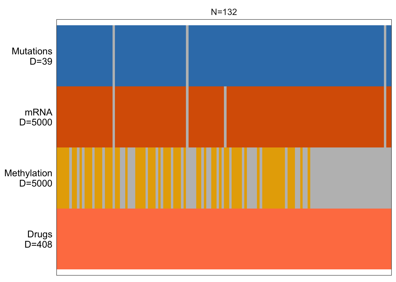
Define MOFA options
Data options
data_opts <- get_default_data_options(MOFAobject)
data_opts
$scale_views
[1] FALSE
$scale_groups
[1] FALSE
$center_groups
[1] TRUE
$use_float32
[1] FALSE
$views
[1] "Drugs" "mRNA" "Mutations" "Methylation"
$groups
[1] "group1"Model options
model_opts <- get_default_model_options(MOFAobject)
model_opts$num_factors <- 10

model_opts
$likelihoods
Drugs mRNA Mutations Methylation
"gaussian" "gaussian" "gaussian" "gaussian"
$num_factors
[1] 10
$spikeslab_factors
[1] FALSE
$spikeslab_weights
[1] TRUE
$ard_factors
[1] FALSE
$ard_weights
[1] TRUEChange the likely hood of Mutations to “bernoulli
model_opts$likelihoods[["Mutations"]] <- "bernoulli"
model_opts$likelihoods
Drugs mRNA Mutations Methylation
"gaussian" "gaussian" "bernoulli" "gaussian" Training options
train_opts <- get_default_training_options(MOFAobject)
train_opts$convergence_mode <- "slow"
train_opts$seed <- 2022
train_opts$maxiter <- 10000
train_opts
$maxiter
[1] 10000
$convergence_mode
[1] "slow"
$drop_factor_threshold
[1] -1
$verbose
[1] FALSE
$startELBO
[1] 1
$freqELBO
[1] 5
$stochastic
[1] FALSE
$gpu_mode
[1] FALSE
$seed
[1] 2022
$outfile
NULL
$weight_views
[1] FALSE
$save_interrupted
[1] FALSEChange drop threshold to 0.01
train_opts$drop_factor_threshold <-0.01Train the MOFA model
Prepare MOFA object
MOFAobject <- prepare_mofa(MOFAobject,
  data_options = data_opts,
  model_options = model_opts,
  training_options = train_opts
)
Checking data options...Checking training options...Checking model options...Training
MOFAobject <- run_mofa(MOFAobject)
saveRDS(MOFAobject,"../output/mofaRes.rds")
Preliminary analysis of the results
MOFAobject <- readRDS("../output/mofaRes.rds")Factor correlation matrix
plot_factor_cor(MOFAobject)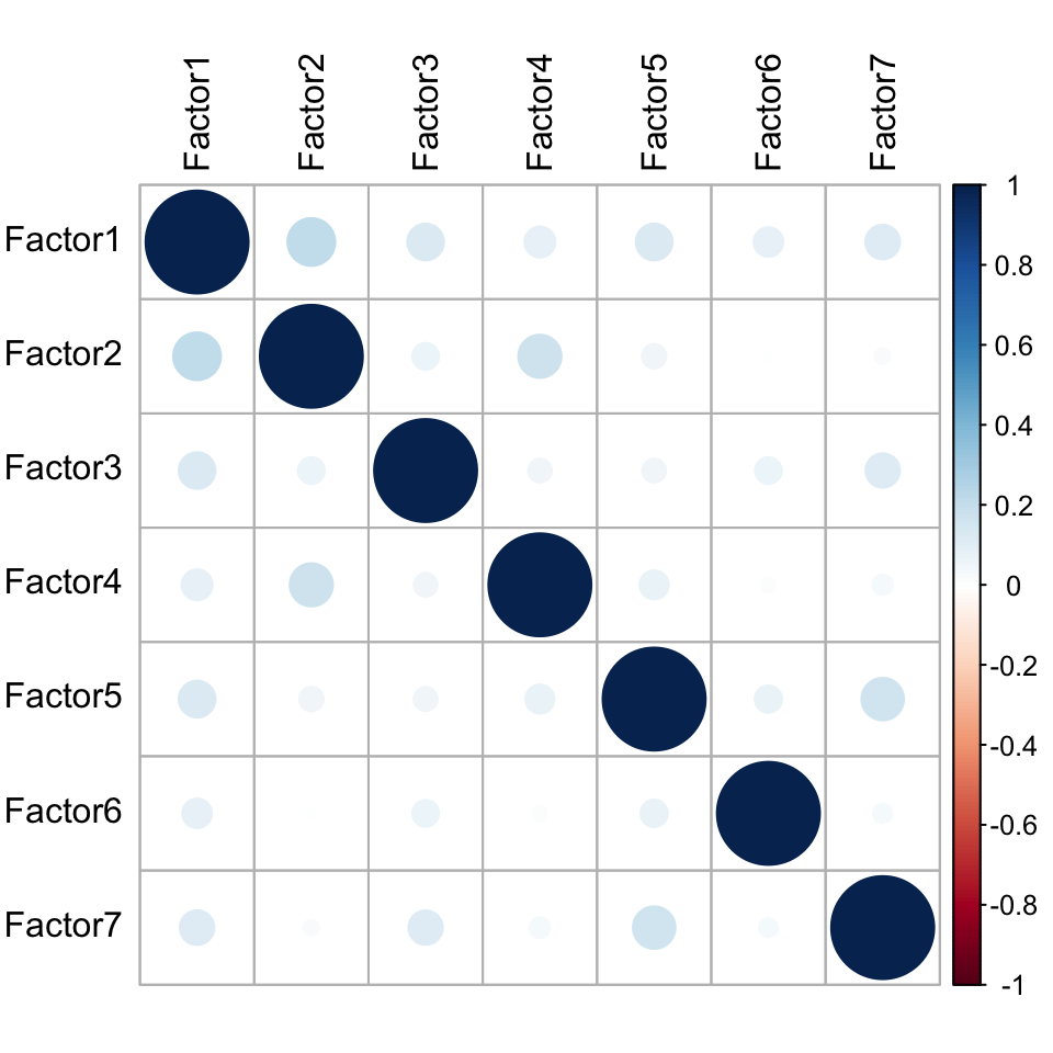
Variance explained
plot_variance_explained(MOFAobject, max_r2=15)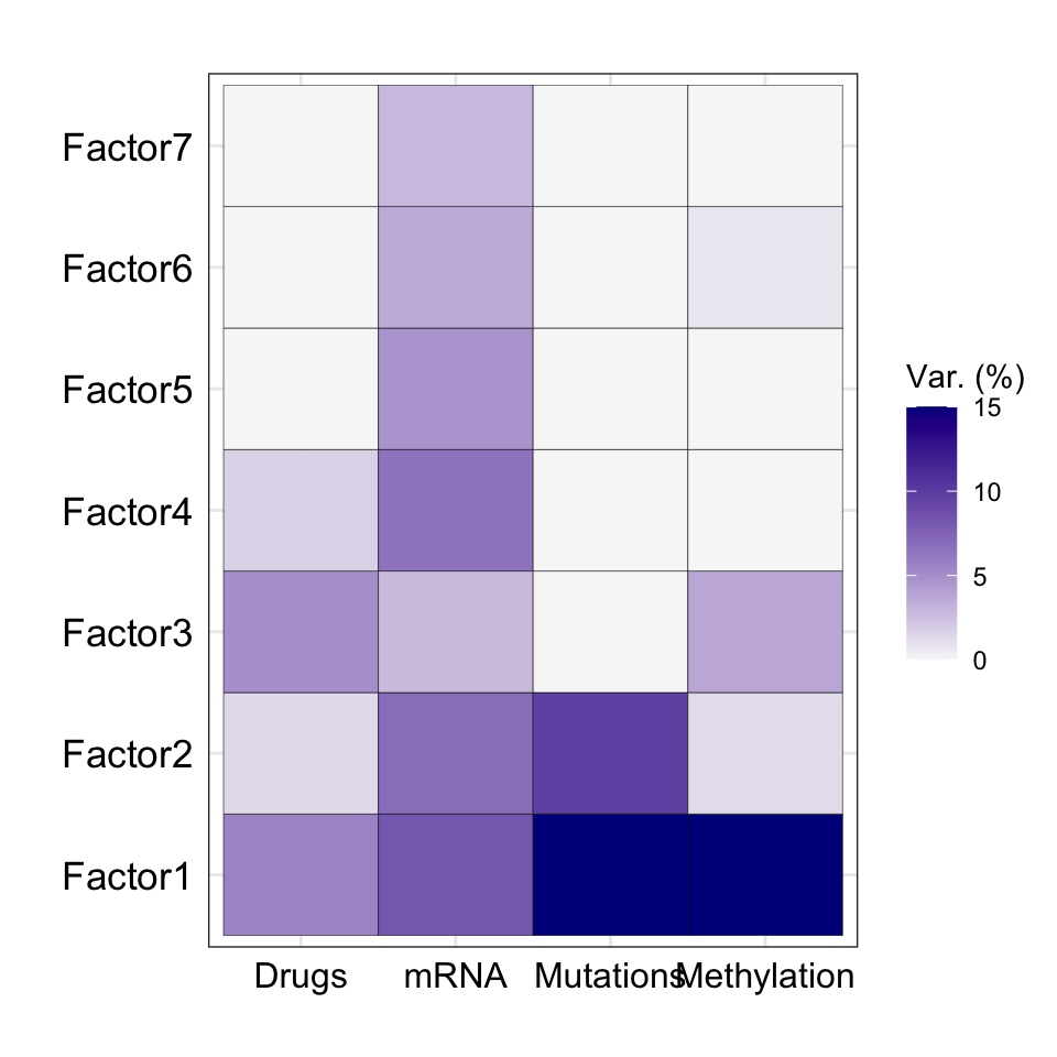 Three factors, F1, F2, F3 and F4, explain variance in the drug
response matrix
Three factors, F1, F2, F3 and F4, explain variance in the drug
response matrix
Total variance explained
plot_variance_explained(MOFAobject, plot_total = T)[[2]]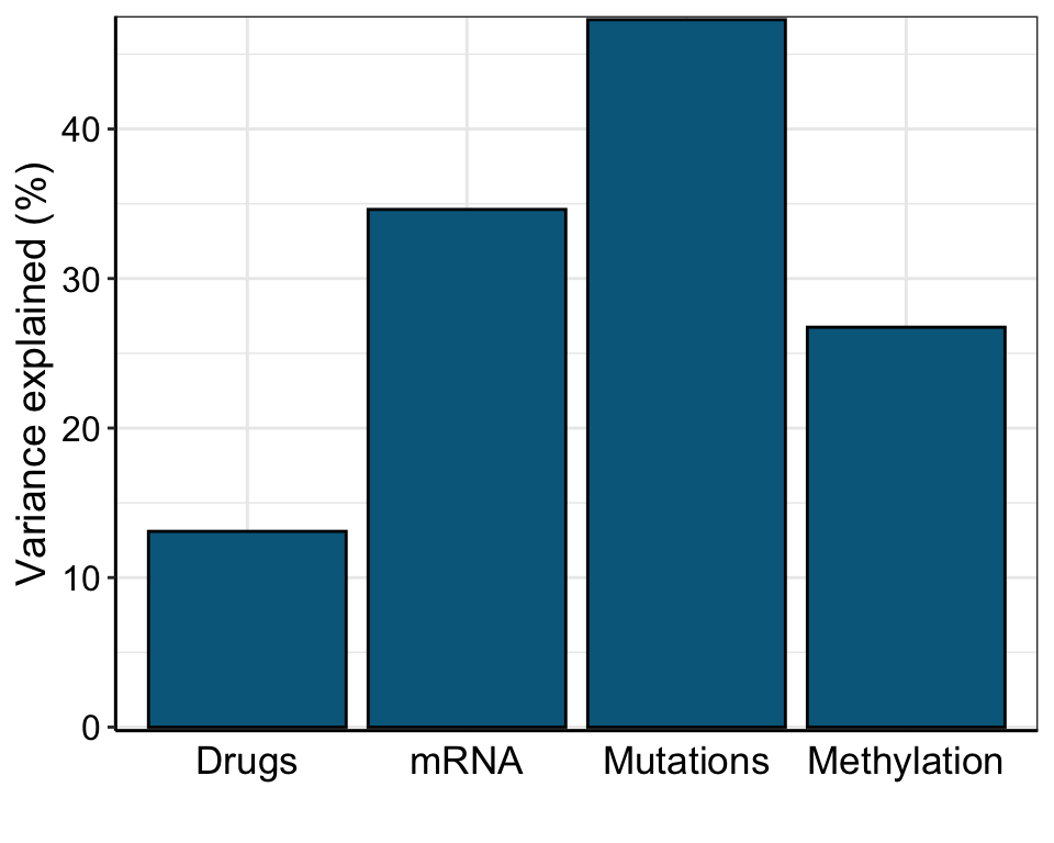
Factor heatmap
library(pheatmap)
#gene annotation
facMat <- t(get_factors(MOFAobject)[[1]])

seleGenes <- c("IGHV", "trisomy12")

colAnno <- tibble(Name = colnames(gene),
                  IGHV = gene["IGHV",],
                  trisomy12 = gene["trisomy12",]) %>%
    column_to_rownames("Name") %>% data.frame()


pheatmap(facMat, clustering_method = "complete", annotation_col = colAnno)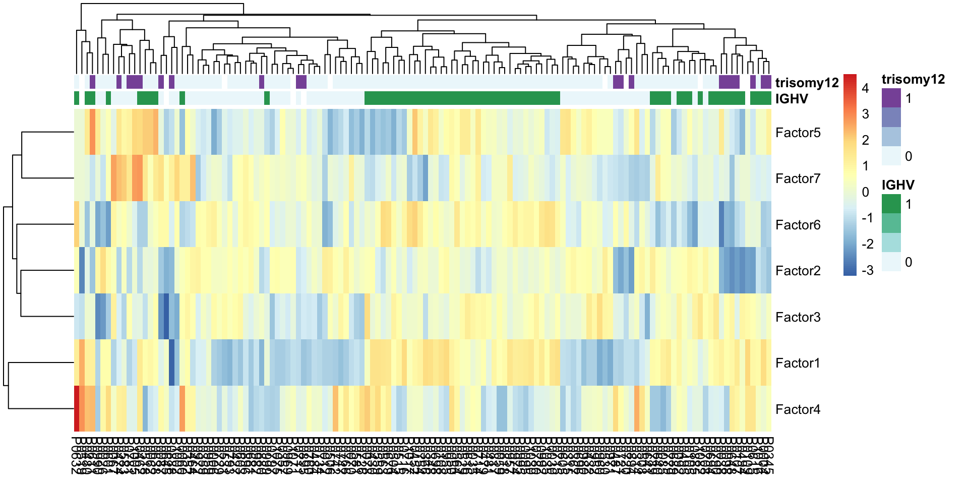
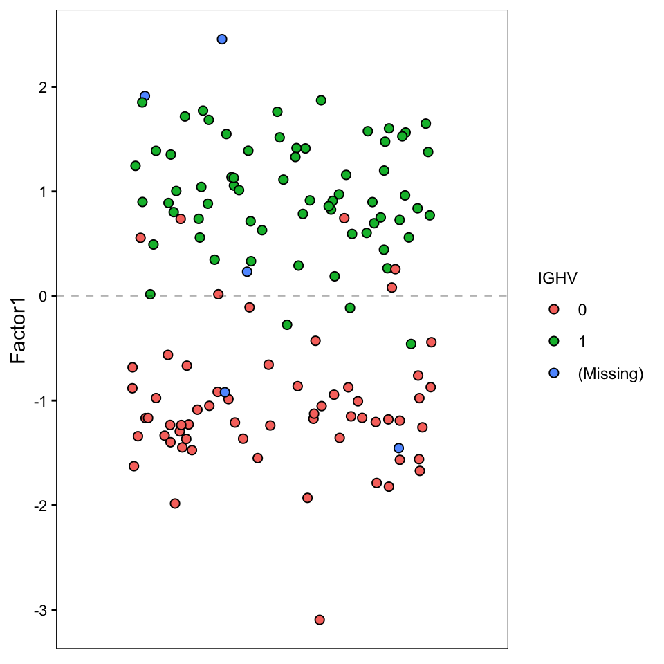
Focus on F1
Factor values
plot_factor(MOFAobject,
  factors = 1,
  color_by = "IGHV"
)
Weight of genomic features
plot_top_weights(MOFAobject,
 view = "Mutations",
 factor = 1,
 nfeatures = 10,     # Top number of features to highlight
 scale = T           # Scale weights from -1 to 1
)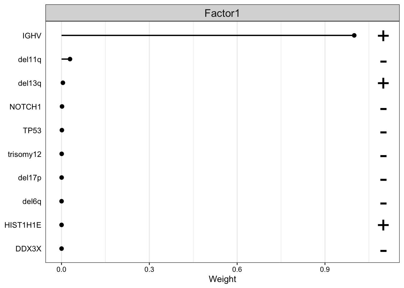
F1 is clearly related to IGHV
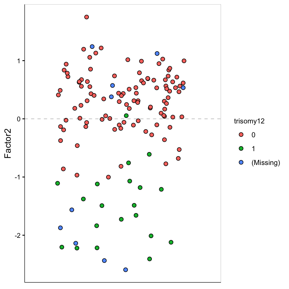
Focus on F2
Factor 2 values
plot_factor(MOFAobject,
  factors = 2,
  color_by = "trisomy12"
)
Weight of genomic features
plot_top_weights(MOFAobject,
view = "Mutations",
factor =2,
nfeatures = 10, # Top number of features to highlight
scale = T # Scale weights from -1 to 1
)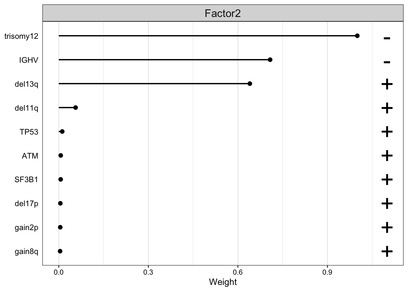 F2 is largely trisomy12
Focus on F3
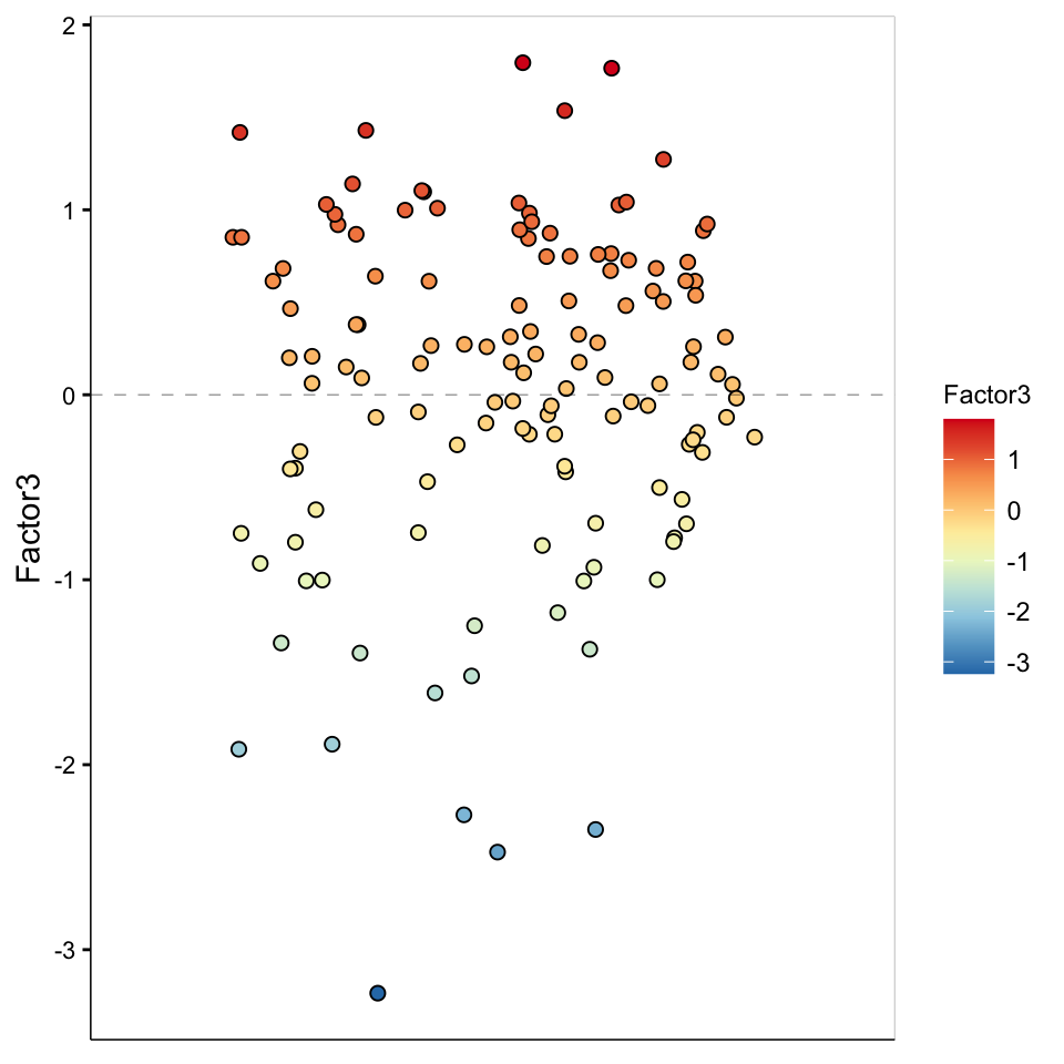
Factor 3 values
plot_factor(MOFAobject,
  factors = 3,
  color_by = "Factor3"
)
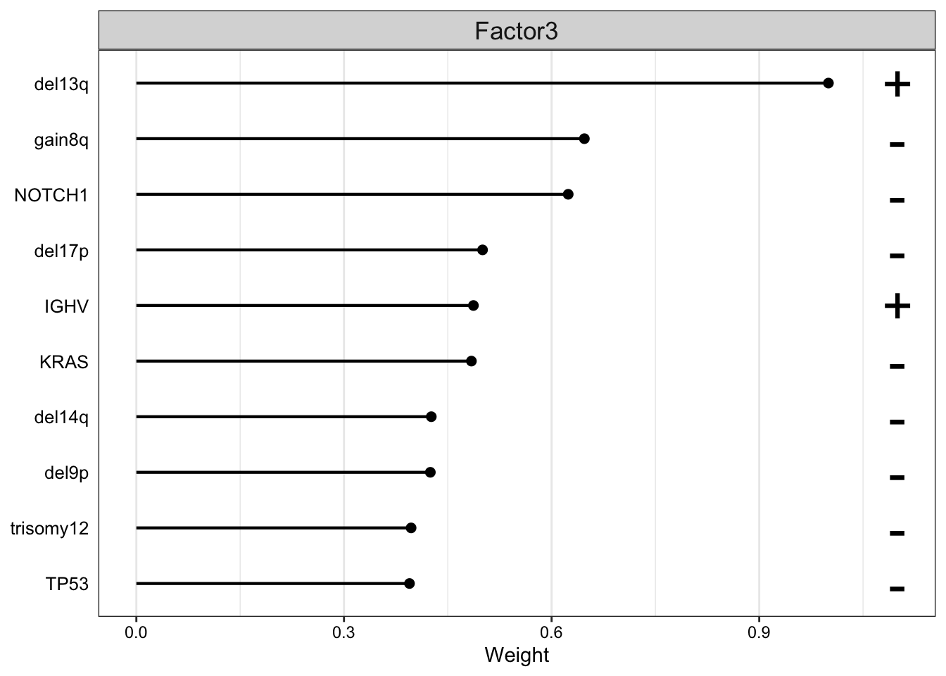
Weight of genomic features on LF3
plot_top_weights(MOFAobject,
 view = "Mutations",
 factor =3,
 nfeatures = 10,     # Top number of features to highlight
 scale = T           # Scale weights from -1 to 1
)
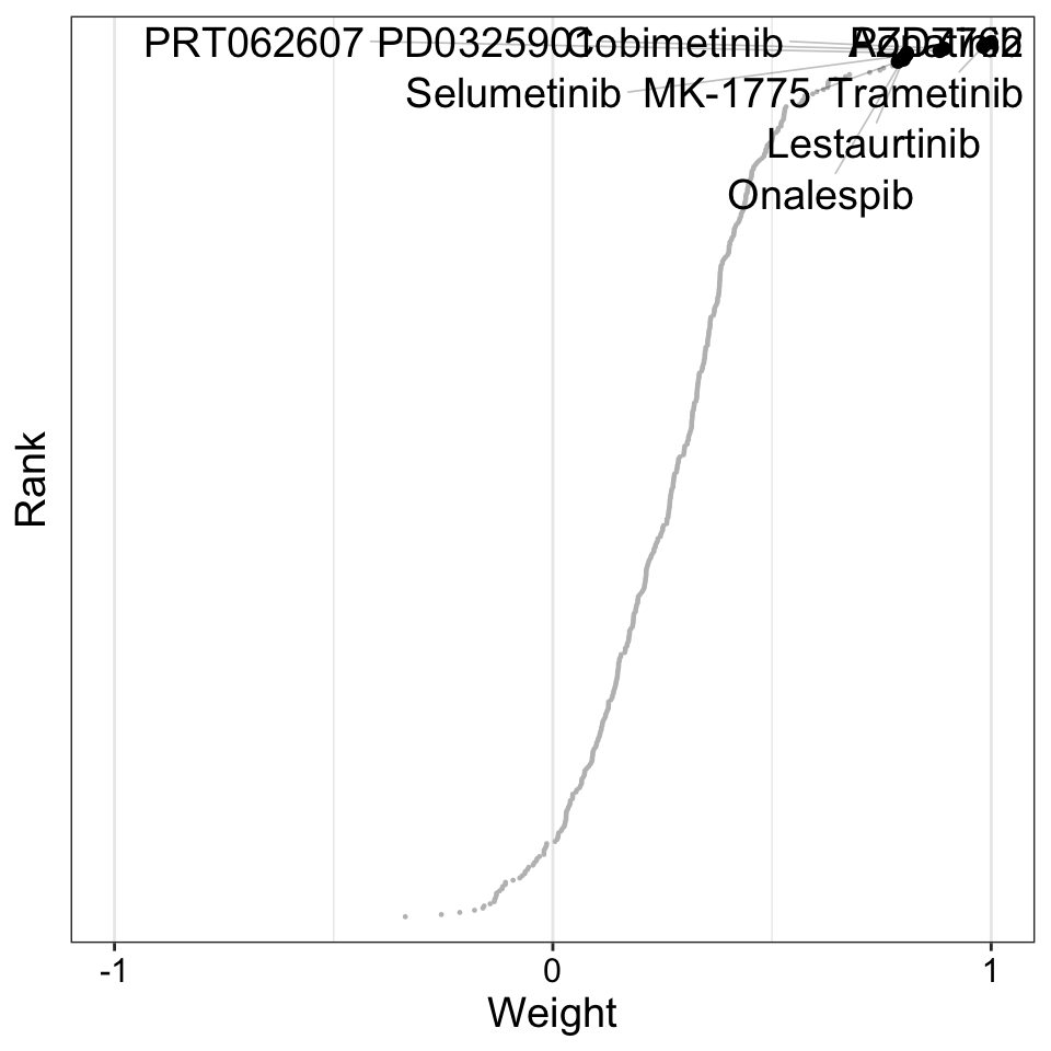
Weight of drug features on LF3
plot_weights(MOFAobject,
 view = "Drugs",
 factor = 3,
 nfeatures = 10,     # Top number of features to highlight
 scale = T           # Scale weights from -1 to 1
)
Associations between F3 and CLL-PD
load("~/CLLproject_jlu/analysis/CLLsubgroup/facTab_methSeqOnly.RData")
comTab <- facTab %>%
    mutate(F3 = facMat["Factor3", match(patID, colnames(facMat))])
ggplot(comTab, aes(x=factor, y=F3)) +
    geom_point() +
    geom_smooth(method = "lm") +
    xlab("CLL-PD")
`geom_smooth()` using formula 'y ~ x'Warning: Removed 148 rows containing non-finite values (stat_smooth).Warning: Removed 148 rows containing missing values (geom_point).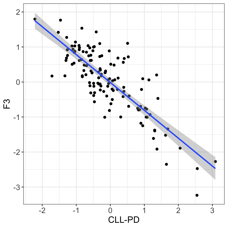
F3 is basically CLL-PD
Focus on F4
F4 only explains variance from drug response and gene expression view
Weight of drug features on LF3
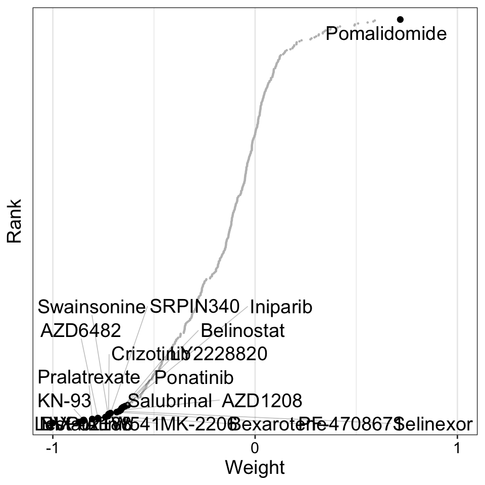
plot_weights(MOFAobject,
 view = "Drugs",
 factor = 4,
 nfeatures = 20,     # Top number of features to highlight
 scale = T           # Scale weights from -1 to 1
)
plot_top_weights(MOFAobject,
view = "Drugs",
factor =4,
nfeatures = 20, # Top number of features to highlight
scale = T # Scale weights from -1 to 1
)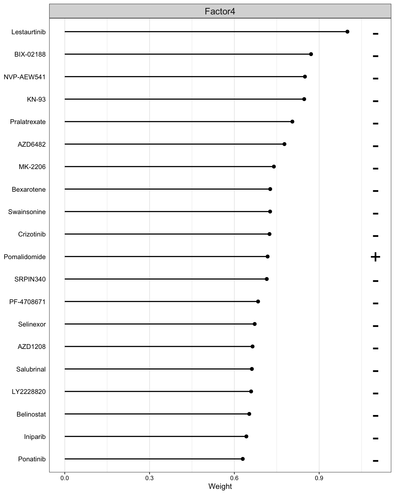 Any interesting drugs?
Association tests between drug responses and F4
library(limma)
Attaching package: 'limma'The following object is masked from 'package:DESeq2':
plotMAThe following object is masked from 'package:BiocGenerics':
plotMAf4 <- facMat["Factor4",]
testMat <- viabMat[,names(f4)]
designMat <- model.matrix(~f4)
fit <- lmFit(testMat, designMat)
fit2 <- eBayes(fit)
resTab <- topTable(fit2, number =Inf)Removing intercept from test coefficientsP value histogram
hist(resTab$P.Value)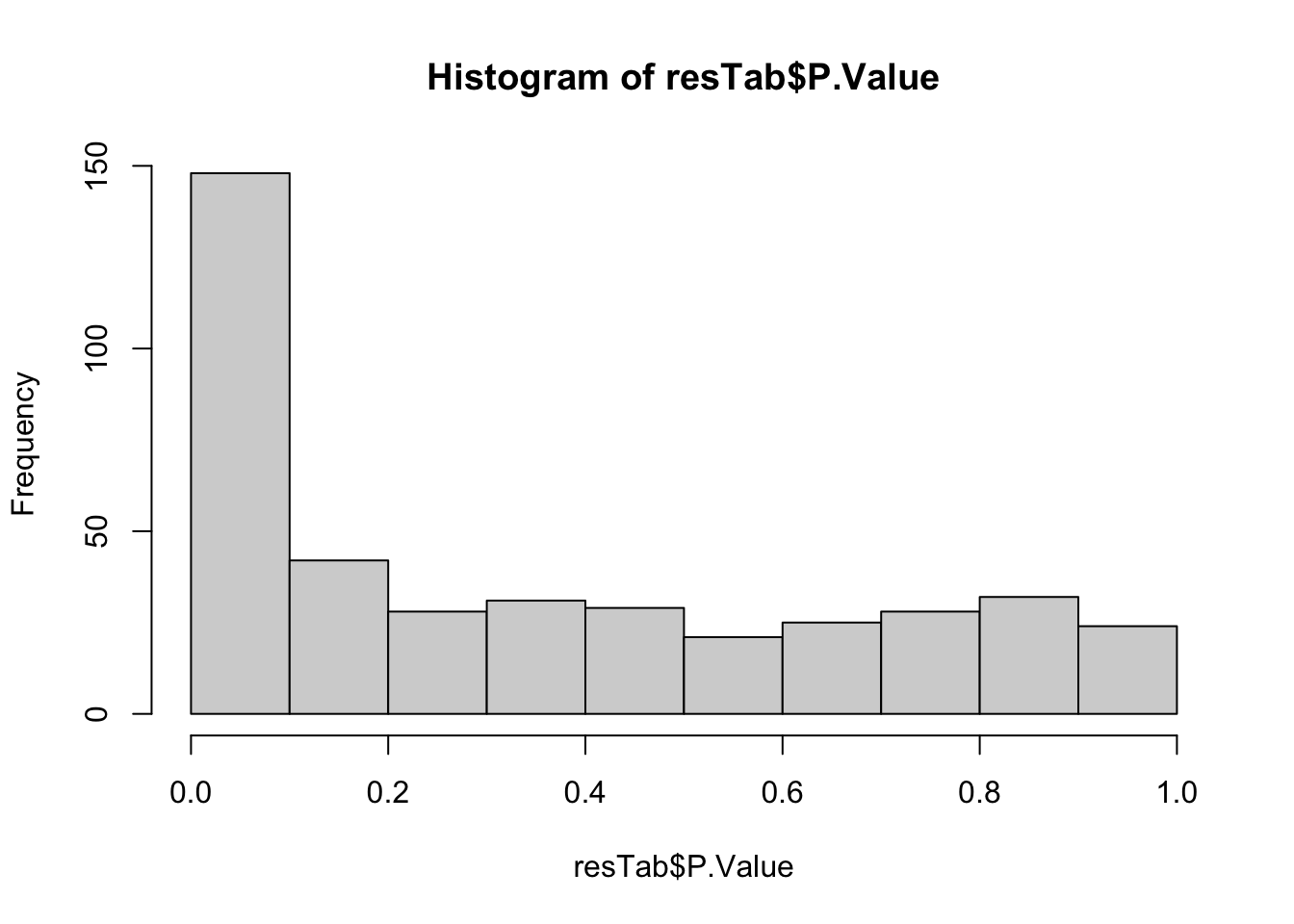
Results passed 10% FDR
resTab.sig <- filter(resTab, adj.P.Val < 0.1) %>%
    as_tibble(rownames = "drugName") %>%
    select(drugName, logFC, P.Value, adj.P.Val) %>%
    left_join(distinct(drugAnno, drugName, target, pathway))
Joining, by = "drugName"resTab.sig %>% mutate_if(is.numeric, formatC, digits=2) %>%
DT::datatable()Scatter plots to visualize top 9 associations
pList <- lapply(seq(9), function(i) {
    rec <- resTab.sig[i,]
    plotTab <- tibble(patID = colnames(viabMat),
                      viab = viabMat[rec$drugName,],
                      F4 = f4,
                      IGHV = gene["IGHV", match(patID, colnames(gene))])
    ggplot(plotTab, aes(x=F4, y=viab)) +
        geom_point(aes(col =factor(IGHV))) + geom_smooth(method = "lm") +
        ggtitle(rec$drugName)
})
cowplot::plot_grid(plotlist = pList, ncol=3)
`geom_smooth()` using formula 'y ~ x'
`geom_smooth()` using formula 'y ~ x'
`geom_smooth()` using formula 'y ~ x'
`geom_smooth()` using formula 'y ~ x'
`geom_smooth()` using formula 'y ~ x'
`geom_smooth()` using formula 'y ~ x'
`geom_smooth()` using formula 'y ~ x'
`geom_smooth()` using formula 'y ~ x'
`geom_smooth()` using formula 'y ~ x'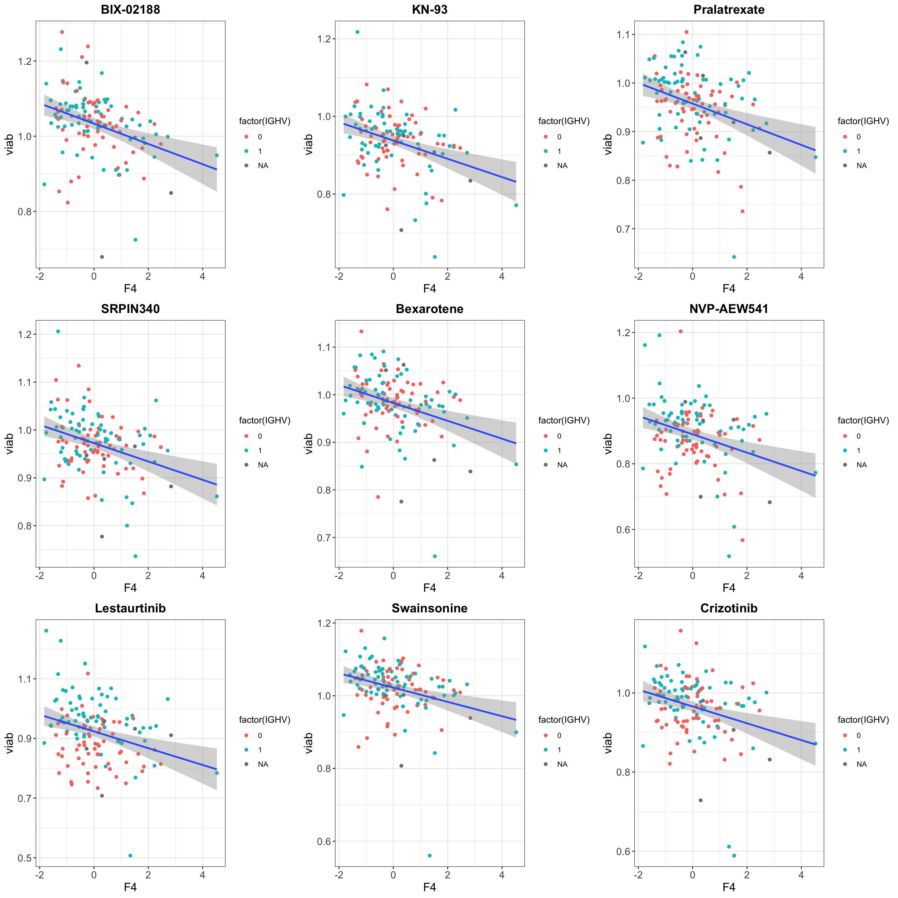
Pathways associated with F4
library(MOFAdata)
data(reactomeGS)
res.positive <- run_enrichment(MOFAobject,
  feature.sets = reactomeGS,
  view = "mRNA",
  sign = "positive"
)
Intersecting features names in the model and the gene set annotation results in a total of 4989 features.
Running feature set Enrichment Analysis with the following options...
View: mRNA
Number of feature sets: 556
Set statistic: mean.diff
Statistical test: parametric
Subsetting weights with positive sign# GSEA on negative weights, with default options
res.negative <- run_enrichment(MOFAobject,
feature.sets = reactomeGS,
view = "mRNA",
sign = "negative"
)Intersecting features names in the model and the gene set annotation results in a total of 4989 features.
Running feature set Enrichment Analysis with the following options...
View: mRNA
Number of feature sets: 556
Set statistic: mean.diff
Statistical test: parametric
Subsetting weights with negative signPositive associations
plot_enrichment(res.positive, factor = 4, max.pathways = 15)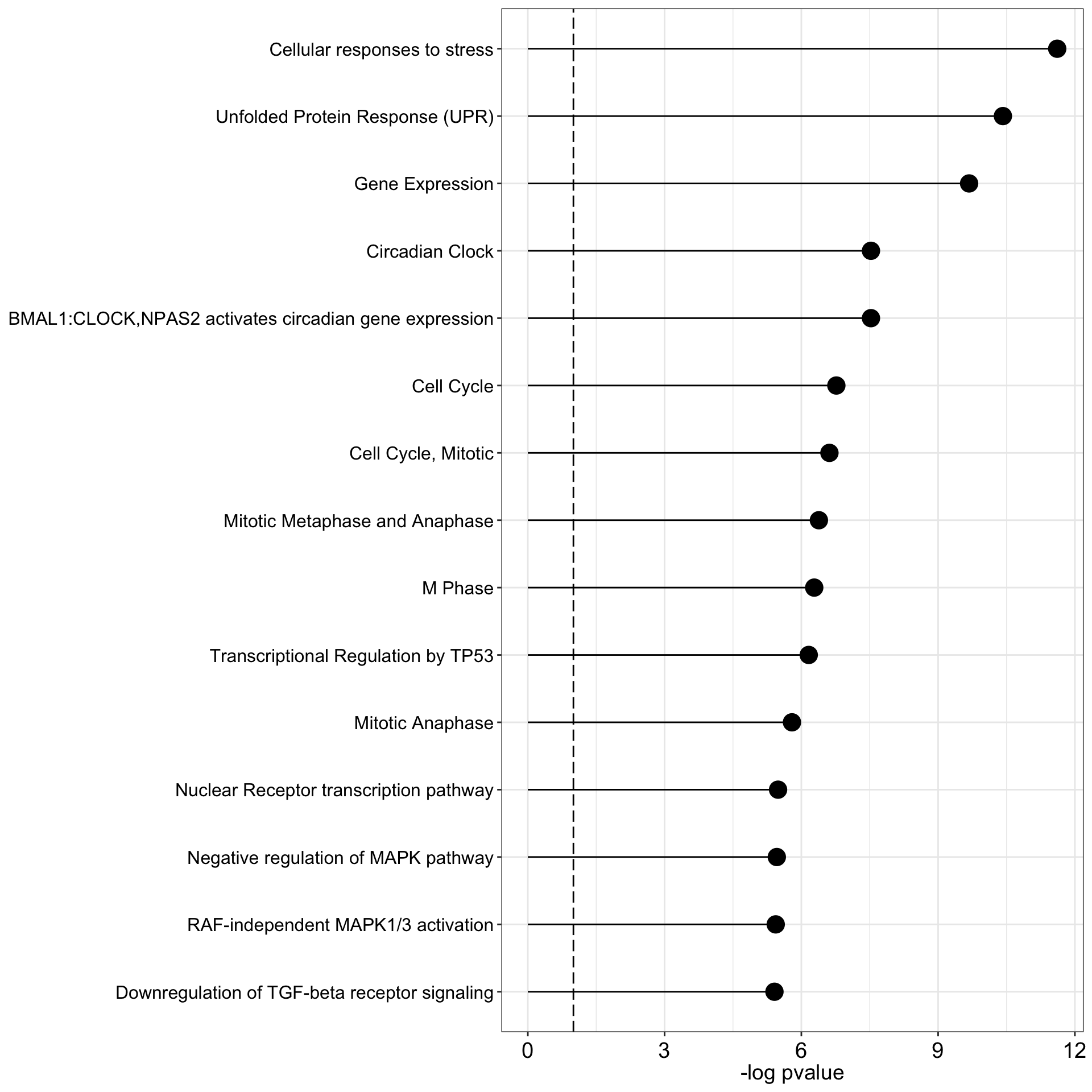 ** F4 is perhaps associated with stress response**
Negative associations
plot_enrichment(res.negative, factor = 4, max.pathways = 15)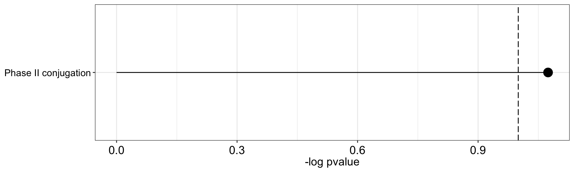
Does F4 associated with baseline ATP levels?
Baseline ATP levels after 48 hours
load("~/CLLproject_jlu/var/newEMBL_20210129.RData")
basalATP <- emblNew %>% filter(type == "neg") %>%
  group_by(patID) %>% summarise(ATPcount = median(val, na.rm=TRUE))
plotTab <- tibble(patID = colnames(facMat),
F4 = facMat["Factor4",]) %>%
left_join(basalATP)Joining, by = "patID"ggplot(plotTab, aes(x=F4, y=ATPcount)) + geom_point() +
geom_smooth(method = "lm")`geom_smooth()` using formula 'y ~ x'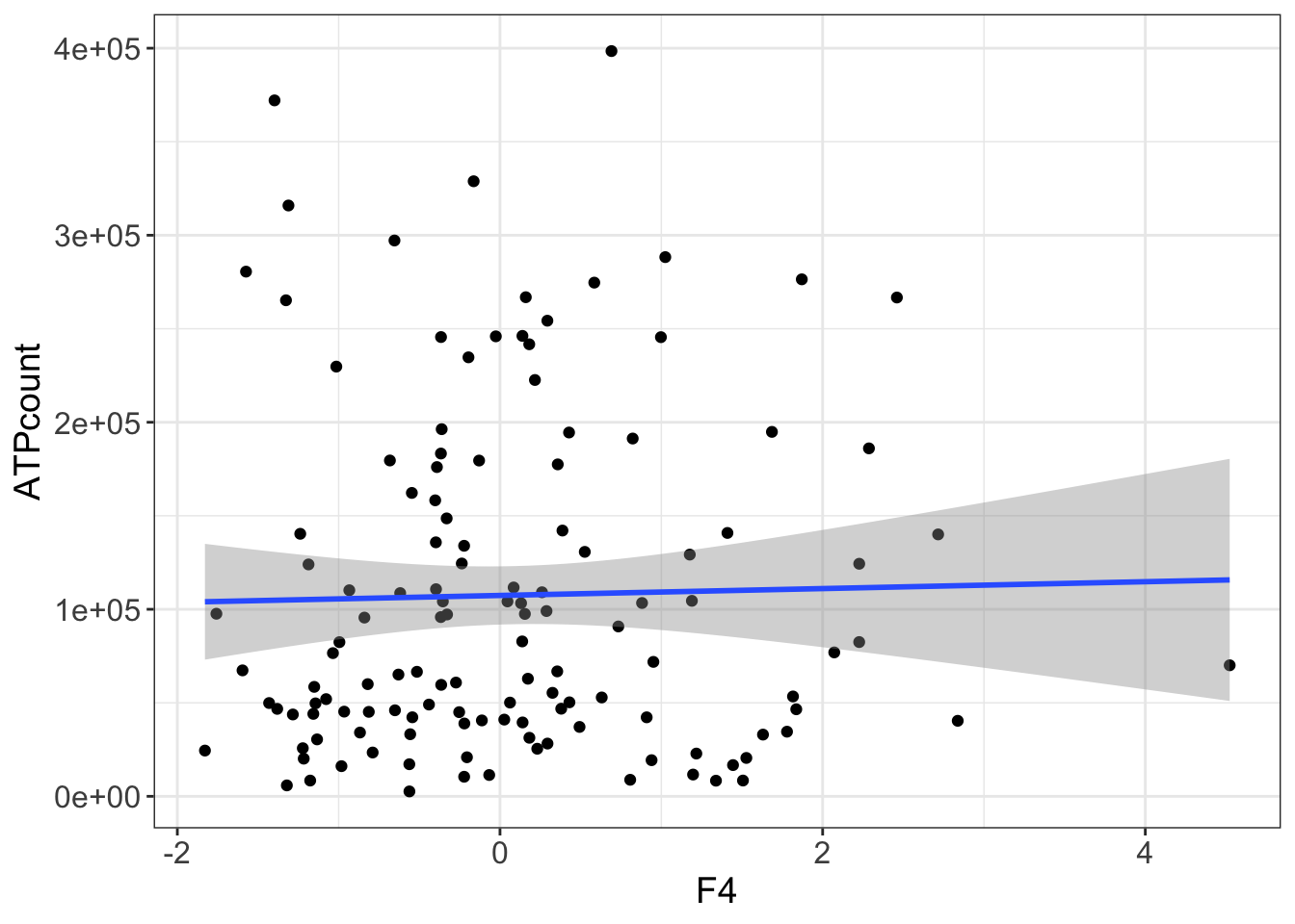 F4 is not associated with baseline ATP.
sessionInfo()R version 4.2.0 (2022-04-22)
Platform: x86_64-apple-darwin17.0 (64-bit)
Running under: macOS Big Sur/Monterey 10.16
Matrix products: default
BLAS: /Library/Frameworks/R.framework/Versions/4.2/Resources/lib/libRblas.0.dylib
LAPACK: /Library/Frameworks/R.framework/Versions/4.2/Resources/lib/libRlapack.dylib
locale:
[1] en_US.UTF-8/en_US.UTF-8/en_US.UTF-8/C/en_US.UTF-8/en_US.UTF-8
attached base packages:
[1] stats4 stats graphics grDevices utils datasets methods
[8] base
other attached packages:
[1] MOFAdata_1.12.0 limma_3.52.2
[3] pheatmap_1.0.12 forcats_0.5.1
[5] stringr_1.4.0 dplyr_1.0.9
[7] purrr_0.3.4 readr_2.1.2
[9] tidyr_1.2.0 tibble_3.1.7
[11] ggplot2_3.3.6 tidyverse_1.3.1
[13] MOFA2_1.6.0 MultiAssayExperiment_1.22.0
[15] sva_3.44.0 BiocParallel_1.30.3
[17] genefilter_1.78.0 mgcv_1.8-40
[19] nlme_3.1-158 DESeq2_1.36.0
[21] SummarizedExperiment_1.26.1 Biobase_2.56.0
[23] MatrixGenerics_1.8.0 matrixStats_0.62.0
[25] GenomicRanges_1.48.0 GenomeInfoDb_1.32.2
[27] IRanges_2.30.0 S4Vectors_0.34.0
[29] BiocGenerics_0.42.0 reticulate_1.25
[31] jyluMisc_0.1.5
loaded via a namespace (and not attached):
[1] utf8_1.2.2 shinydashboard_0.7.2 tidyselect_1.1.2
[4] RSQLite_2.2.14 AnnotationDbi_1.58.0 htmlwidgets_1.5.4
[7] grid_4.2.0 Rtsne_0.16 maxstat_0.7-25
[10] munsell_0.5.0 codetools_0.2-18 DT_0.23
[13] withr_2.5.0 colorspace_2.0-3 filelock_1.0.2
[16] highr_0.9 knitr_1.39 rstudioapi_0.13
[19] ggsignif_0.6.3 labeling_0.4.2 git2r_0.30.1
[22] slam_0.1-50 GenomeInfoDbData_1.2.8 KMsurv_0.1-5
[25] farver_2.1.0 bit64_4.0.5 rhdf5_2.40.0
[28] rprojroot_2.0.3 basilisk_1.8.0 vctrs_0.4.1
[31] generics_0.1.2 TH.data_1.1-1 xfun_0.31
[34] sets_1.0-21 R6_2.5.1 locfit_1.5-9.5
[37] bitops_1.0-7 rhdf5filters_1.8.0 cachem_1.0.6
[40] fgsea_1.22.0 DelayedArray_0.22.0 assertthat_0.2.1
[43] promises_1.2.0.1 scales_1.2.0 multcomp_1.4-19
[46] gtable_0.3.0 sandwich_3.0-2 workflowr_1.7.0
[49] rlang_1.0.2 splines_4.2.0 rstatix_0.7.0
[52] broom_0.8.0 modelr_0.1.8 yaml_2.3.5
[55] reshape2_1.4.4 abind_1.4-5 crosstalk_1.2.0
[58] backports_1.4.1 httpuv_1.6.5 tools_4.2.0
[61] relations_0.6-12 ellipsis_0.3.2 gplots_3.1.3
[64] jquerylib_0.1.4 RColorBrewer_1.1-3 Rcpp_1.0.8.3
[67] plyr_1.8.7 visNetwork_2.1.0 zlibbioc_1.42.0
[70] RCurl_1.98-1.7 basilisk.utils_1.8.0 ggpubr_0.4.0
[73] cowplot_1.1.1 zoo_1.8-10 haven_2.5.0
[76] ggrepel_0.9.1 cluster_2.1.3 exactRankTests_0.8-35
[79] fs_1.5.2 magrittr_2.0.3 data.table_1.14.2
[82] reprex_2.0.1 survminer_0.4.9 mvtnorm_1.1-3
[85] hms_1.1.1 shinyjs_2.1.0 mime_0.12
[88] evaluate_0.15 xtable_1.8-4 XML_3.99-0.10
[91] readxl_1.4.0 gridExtra_2.3 compiler_4.2.0
[94] KernSmooth_2.23-20 crayon_1.5.1 htmltools_0.5.2
[97] tzdb_0.3.0 later_1.3.0 geneplotter_1.74.0
[100] lubridate_1.8.0 DBI_1.1.3 corrplot_0.92
[103] dbplyr_2.2.0 MASS_7.3-57 Matrix_1.4-1
[106] car_3.1-0 cli_3.3.0 marray_1.74.0
[109] parallel_4.2.0 igraph_1.3.2 pkgconfig_2.0.3
[112] km.ci_0.5-6 dir.expiry_1.4.0 piano_2.12.0
[115] xml2_1.3.3 annotate_1.74.0 bslib_0.3.1
[118] XVector_0.36.0 drc_3.0-1 rvest_1.0.2
[121] digest_0.6.29 Biostrings_2.64.0 cellranger_1.1.0
[124] rmarkdown_2.14 fastmatch_1.1-3 survMisc_0.5.6
[127] uwot_0.1.11 edgeR_3.38.1 shiny_1.7.1
[130] gtools_3.9.2.2 lifecycle_1.0.1 jsonlite_1.8.0
[133] Rhdf5lib_1.18.2 carData_3.0-5 fansi_1.0.3
[136] pillar_1.7.0 lattice_0.20-45 KEGGREST_1.36.2
[139] fastmap_1.1.0 httr_1.4.3 plotrix_3.8-2
[142] survival_3.3-1 glue_1.6.2 png_0.1-7
[145] bit_4.0.4 stringi_1.7.6 sass_0.4.1
[148] HDF5Array_1.24.1 blob_1.2.3 caTools_1.18.2
[151] memoise_2.0.1