Consensus clustering analysis based on drug responses (CPS1000)
Junyan Lu
6 April 2022
Last updated: 2022-04-06
Checks: 6 1
Knit directory: EMBL2016/analysis/
This reproducible R Markdown analysis was created with workflowr (version 1.7.0). The Checks tab describes the reproducibility checks that were applied when the results were created. The Past versions tab lists the development history.
The R Markdown is untracked by Git. To know which version of the R Markdown file created these results, you’ll want to first commit it to the Git repo. If you’re still working on the analysis, you can ignore this warning. When you’re finished, you can run wflow_publish to commit the R Markdown file and build the HTML.
Great job! The global environment was empty. Objects defined in the global environment can affect the analysis in your R Markdown file in unknown ways. For reproduciblity it’s best to always run the code in an empty environment.
The command set.seed(20210512) was run prior to running the code in the R Markdown file. Setting a seed ensures that any results that rely on randomness, e.g. subsampling or permutations, are reproducible.
Great job! Recording the operating system, R version, and package versions is critical for reproducibility.
Nice! There were no cached chunks for this analysis, so you can be confident that you successfully produced the results during this run.
Great job! Using relative paths to the files within your workflowr project makes it easier to run your code on other machines.
Great! You are using Git for version control. Tracking code development and connecting the code version to the results is critical for reproducibility.
The results in this page were generated with repository version 12d1722. See the Past versions tab to see a history of the changes made to the R Markdown and HTML files.
Note that you need to be careful to ensure that all relevant files for the analysis have been committed to Git prior to generating the results (you can use wflow_publish or wflow_git_commit). workflowr only checks the R Markdown file, but you know if there are other scripts or data files that it depends on. Below is the status of the Git repository when the results were generated:
Ignored files:
    Ignored:    .DS_Store
    Ignored:    .Rhistory
    Ignored:    analysis/.DS_Store
    Ignored:    analysis/.Rhistory
    Ignored:    analysis/boxplot_AUC.png
    Ignored:    analysis/consensus_clustering_noFit_cache/
    Ignored:    analysis/dose_curve.png
    Ignored:    analysis/targetDist.png
    Ignored:    analysis/toxivity_box.png
    Ignored:    analysis/volcano.png
    Ignored:    data/.DS_Store

Untracked files:
    Untracked:  analysis/AUC_CLL_IC50/
    Untracked:  analysis/BRAF_analysis.Rmd
    Untracked:  analysis/GSVA_analysis.Rmd
    Untracked:  analysis/NOTCH1_signature.Rmd
    Untracked:  analysis/autoluminescence.Rmd
    Untracked:  analysis/bar_plot_mixed.pdf
    Untracked:  analysis/bar_plot_mixed_noU1.pdf
    Untracked:  analysis/beatAML/
    Untracked:  analysis/cohortComposition_CLLsamples.pdf
    Untracked:  analysis/cohortComposition_allSamples.pdf
    Untracked:  analysis/consensus_clustering.Rmd
    Untracked:  analysis/consensus_clustering_CPS.Rmd
    Untracked:  analysis/consensus_clustering_IC50.Rmd
    Untracked:  analysis/consensus_clustering_beatAML.Rmd
    Untracked:  analysis/consensus_clustering_noFit.Rmd
    Untracked:  analysis/consensus_clusters.pdf
    Untracked:  analysis/disease_specific.Rmd
    Untracked:  analysis/dose_curve_selected.pdf
    Untracked:  analysis/genomic_association.Rmd
    Untracked:  analysis/genomic_association_allDisease.Rmd
    Untracked:  analysis/mean_autoluminescence_val.csv
    Untracked:  analysis/mean_autoluminescence_val.xlsx
    Untracked:  analysis/noFit_CLL/
    Untracked:  analysis/number_associations.pdf
    Untracked:  analysis/overview.Rmd
    Untracked:  analysis/plotCohort.Rmd
    Untracked:  analysis/preprocess.Rmd
    Untracked:  analysis/volcano_noBlocking.pdf
    Untracked:  code/utils.R
    Untracked:  data/BeatAML_Waves1_2/
    Untracked:  data/ic50Tab.RData
    Untracked:  data/newEMBL_20210806.RData
    Untracked:  data/patMeta.RData
    Untracked:  data/targetAnnotation_all.csv
    Untracked:  force_sync.sh
    Untracked:  output/resConsClust.RData
    Untracked:  output/resConsClust_aucFit.RData
    Untracked:  output/resConsClust_beatAML.RData
    Untracked:  output/resConsClust_cps.RData
    Untracked:  output/resConsClust_ic50.RData
    Untracked:  output/resConsClust_noFit.RData
    Untracked:  output/screenData.RData
    Untracked:  sync.sh

Unstaged changes:
    Modified:   _workflowr.yml
    Modified:   analysis/_site.yml
    Deleted:    analysis/about.Rmd
    Modified:   analysis/index.Rmd
    Deleted:    analysis/license.Rmd
Note that any generated files, e.g. HTML, png, CSS, etc., are not included in this status report because it is ok for generated content to have uncommitted changes.
There are no past versions. Publish this analysis with wflow_publish() to start tracking its development.
Load libraries and datasets
Perform consensus clustering to identify CLL subgroups with different drug response pattern
Pre-processing
Select CLL samples and use AUC as measures of drug effect
screenData <- pheno1000_main %>% dplyr::rename(viab = normVal.adj.sigm, viab.auc  = normVal.adj.cor_auc, conc = Concentration)
#Prepare data
viabMat <- screenData %>%
  filter(diagnosis %in% "CLL") %>% #only CLL
  group_by(patientID, Drug) %>% summarise(viab = mean(viab.auc, na.rm=TRUE)) %>%
  spread(key = patientID, value = "viab") %>% data.frame() %>%
  column_to_rownames("Drug") %>% as.matrix()
Estimate missing value percentage
missDrug <- rowSums(is.na(viabMat))
missPat <- colSums(is.na(viabMat))
Original dimension
dim(viabMat)[1] 65 275Keep drug that have non-NA values in at least 80% of samples
viabMatFilt <- viabMat[missDrug/ncol(viabMat) <= 0.2, ]Number of filtered dimensions
dim(viabMatFilt)[1] 63 275Run clustering with ConcsensusClustterPlus
# Impute missing values using missForest, as missing values are not allowed for consensus clustering
viabMatImp <- viabMatFilt
#Center each feature by median
d <- sweep(viabMatImp,1, apply(viabMatImp,1, median, na.rm=T))
#consensus clustering
resConsClust <- ConsensusClusterPlus(d, maxK=20, reps=1000, pItem=0.8, pFeature=1, title = "AUC_CLL_CPS",
clusterAlg="hc",distance="pearson",seed=2021, plot="png")
#plot clustering result
#icl = calcICL(resConsClust,title="AUC_CLL_CPS1000",plot="png")
#save results for later use
save(viabMatImp, resConsClust, file = "../output/resConsClust_cps.RData")Based on delta curve, three clusters would be most appropriate
load("../output/resConsClust_cps.RData")Post-processing consensus clustering results
Select samples with clustering consensus over 80%
k=3
conMat <- resConsClust[[k]]$consensusMatrix
conClust <- resConsClust[[k]]$consensusClass
colnames(conMat) <- colnames(viabMatImp)

#change cluster number to be consistent with EMBL screen reuslts
conClust <- case_when(conClust == 1 ~ 2,
                      conClust == 2 ~ 3,
                      conClust == 3 ~ 1)
names(conClust) <- colnames(conMat)
Visualization
clusterTab <- tibble(patientID = colnames(conMat),
                      cluster = paste0("C",conClust),
                      IGHV.status = patMeta[match(names(conClust),patMeta$Patient.ID),]$IGHV.status,
                      Mclust = patMeta[match(names(conClust),patMeta$Patient.ID),]$Methylation_Cluster,
                      trisomy12 = patMeta[match(names(conClust),patMeta$Patient.ID),]$trisomy12)

colAnno <- clusterTab %>% data.frame() %>% column_to_rownames("patientID")
pheatmap(conMat, annotation_col = colAnno, method = "average", clustering_distance_rows = "correlation", clustering_distance_cols = "correlation")
Based on the heatmap, C2 is primarily U-CLL samples while C1 and C2 are primarily M-CLL samples
Visualization (for abstract)
colAnnoAlt <- data.frame(row.names = colnames(conMat),
                      cluster = paste0("C",conClust),
                      IGHV.status = patMeta[match(names(conClust),patMeta$Patient.ID),]$IGHV.status)

annoCol <- list(IGHV.status = c(M = "#E41A1C", U = "#377EB8"),
                cluster = c(C1 = "#4DAF4A", C2 = "#984EA3", C3 = "#FF7F00"))
#pdf("consensus_clusters.pdf", height = 4, width = 5)
pheatmap(conMat, annotation_col = colAnnoAlt, method = "average", clustering_distance_rows = "correlation", clustering_distance_cols = "correlation",
         color = blues9, treeheight_row = 0, treeheight_col = 1, border_color = NA, show_colnames = FALSE, annotation_colors = annoCol)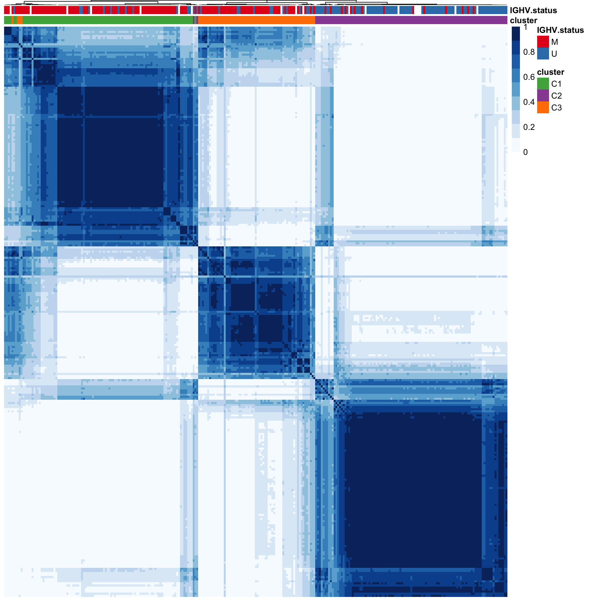
#dev.off()C1 and C3 groups are predominately M-CLL samples
table(clusterTab$cluster, clusterTab$IGHV.status)
      M  U
  C1 81 12
  C2 14 84
  C3 52 13
plotTab <- clusterTab %>%
filter(!is.na(IGHV.status)) %>%
group_by(cluster, IGHV.status) %>%
summarise(n=length(patientID))
ggplot(plotTab, aes(x=cluster,y=n, fill = IGHV.status)) +
geom_bar(stat="identity", postion = "stack") +
xlab("number of samples") +
scale_fill_manual(values = c(M = "#E41A1C", U = "#377EB8")) +
theme_my +
theme(legend.position = "bottom")
C1 and C3 groups are predominately M-CLL samples
table(clusterTab$cluster, clusterTab$Mclust)
     HP IP LP
  C1 69 10 12
  C2 10  6 81
  C3 34 20  6
plotTab <- clusterTab %>%
filter(!is.na(Mclust)) %>%
group_by(cluster, Mclust) %>%
summarise(n=length(patientID))
ggplot(plotTab, aes(x=cluster,y=n, fill = Mclust)) +
geom_bar(stat="identity", postion = "stack") +
xlab("number of samples") +
#scale_fill_manual(values = c(M = "#E41A1C", U = "#377EB8")) +
theme_my +
theme(legend.position = "bottom")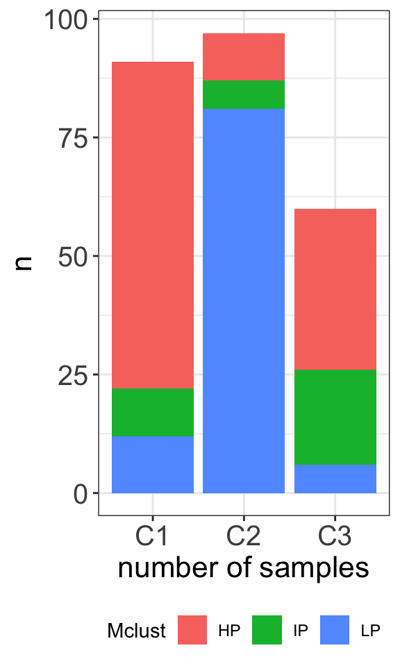
Both C1 and C3 are M-CLL samples. How they are different in terms of drug responses and why they are different?
T-SNE visualization
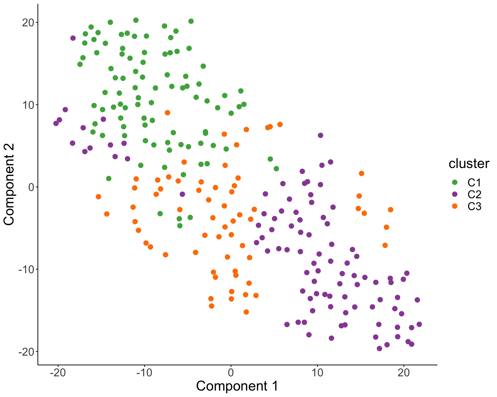
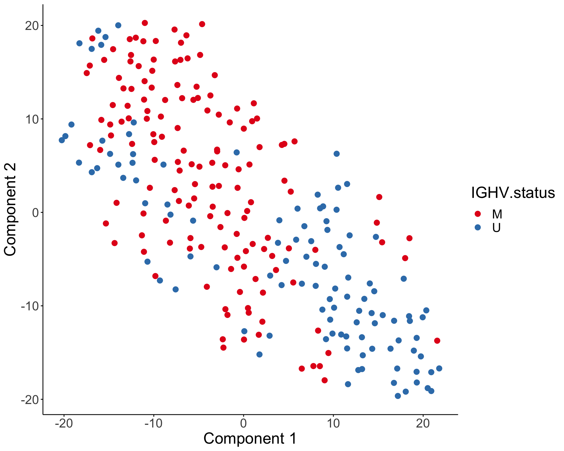
Characterize the drug response phenotypes of C1 and C3 subgroup within M-CLL samples
In this part, I want to answer the question how C1 and C3 subgroups are different in terms of drug response profile. As samples in C1 and C3 group are primarily M-CLL samples, in the analysis below, only M-CLL samples will be considered.
Identify drugs that show differential responses between C1 and C3 in M-CLL samples
clusterTab <- clusterTab %>%
  mutate(sampleID = screenData[match(patientID, screenData$patientID),]$sampleID)

testTabAll <- screenData %>%
  filter(diagnosis %in% "CLL") %>% #only CLL
  group_by(patientID, Drug) %>% summarise(viab = mean(viab.auc, na.rm=TRUE)) %>%
  left_join(clusterTab, by = "patientID")

testTab <- testTabAll %>%
  filter(cluster %in% c("C1","C3"),
         IGHV.status %in% "M",
         !is.na(viab)) %>%
  mutate(cluster =factor(cluster, levels = c("C1","C3")))

#at least five samples if each cluster for each drug, this is because for some drugs the AUC could not be fitted
drugFilt <- group_by(testTab, cluster, Drug) %>%
  summarise(n = length(!is.na(viab))) %>%
  pivot_wider(names_from = cluster, values_from = n) %>%
  filter(C1>=5 & C3>=5)

testTab <- filter(testTab, Drug %in% drugFilt$Drug)
resTab <- testTab %>% group_by(Drug) %>% nest() %>%
mutate(m=map(data, ~t.test(viab~cluster, ., var.equal=TRUE))) %>%
mutate(res = map(m, broom::tidy)) %>%
unnest(res) %>% ungroup() %>%
select(Drug, estimate, p.value, estimate1, estimate2) %>%
mutate(p.adj = p.adjust(p.value, method = "BH"), log2FC = log2(estimate2/estimate1)) %>%
arrange(p.value)Volcano plot
plotTabVol <- resTab %>%
  mutate(direction = case_when(p.adj > 0.01 ~ "n.s.",
                               p.adj < 0.01 & log2FC <0 ~ "sensitive in C3",
                               p.adj < 0.01 & log2FC >0 ~ "resistent in C3"))

#label top 12 drugs judged by pvalue
topDrug <- arrange(resTab, p.value)$Drug[1:12]
plotTabVol <- mutate(plotTabVol, drugLabel = ifelse(Drug %in% topDrug, as.character(Drug), ""))

ggplot(plotTabVol, aes(y=-log10(p.adj), x= log2FC)) +
  geom_point(aes(col = direction)) +
  geom_hline(yintercept = 2, linetype ="dashed") +
  ggrepel::geom_text_repel(aes(label = drugLabel),max.overlaps=100) +
  scale_color_manual(values = c(n.s. = "grey50", `sensitive in C3` = "blue", `resistent in C3` = "red")) +
  xlim(-0.8,0.8) +
  ggtitle("Drug sensitivity between C1 and C3\n(within M-CLL samples)") +
  theme_my +
  theme(plot.title = element_text(hjust=0.5, size=15, face ="bold"))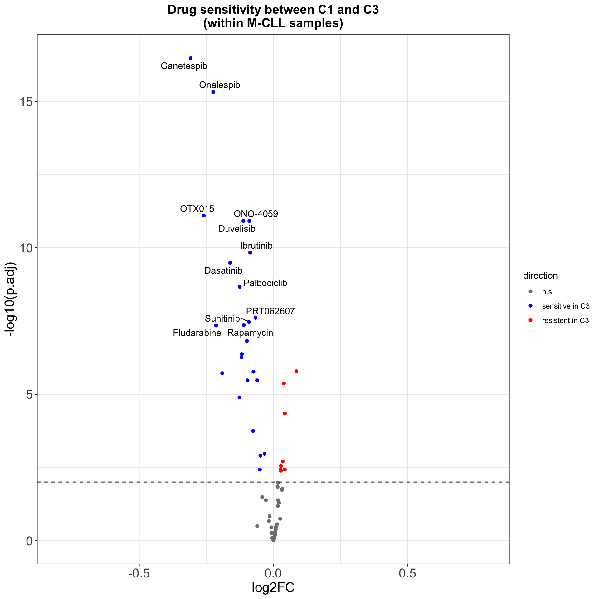
ggsave("volcano.png", height = 5, width = 6)Drug with 1% FDR and abs(log2FC) > 0.5 are labeled
A list of all drugs associated with C1/C3 subgroups
10% FDR cut-off is used
resTab %>% filter(p.adj < 0.1) %>%
  mutate_if(is.numeric, formatC, digits=2) %>%
  DT::datatable()
Boxplots
Only M-CLL samples that belong to C1 and C3 group
drugList <- filter(plotTabVol, drugLabel != "")$Drug
plotTabBox <- filter(testTab, Drug %in% drugList)
ggplot(plotTabBox, aes(x=cluster, y = viab)) +
  geom_boxplot(outlier.shape = NA, aes(fill = cluster)) + ggbeeswarm::geom_quasirandom() +
  facet_wrap(~Drug) +
  theme_my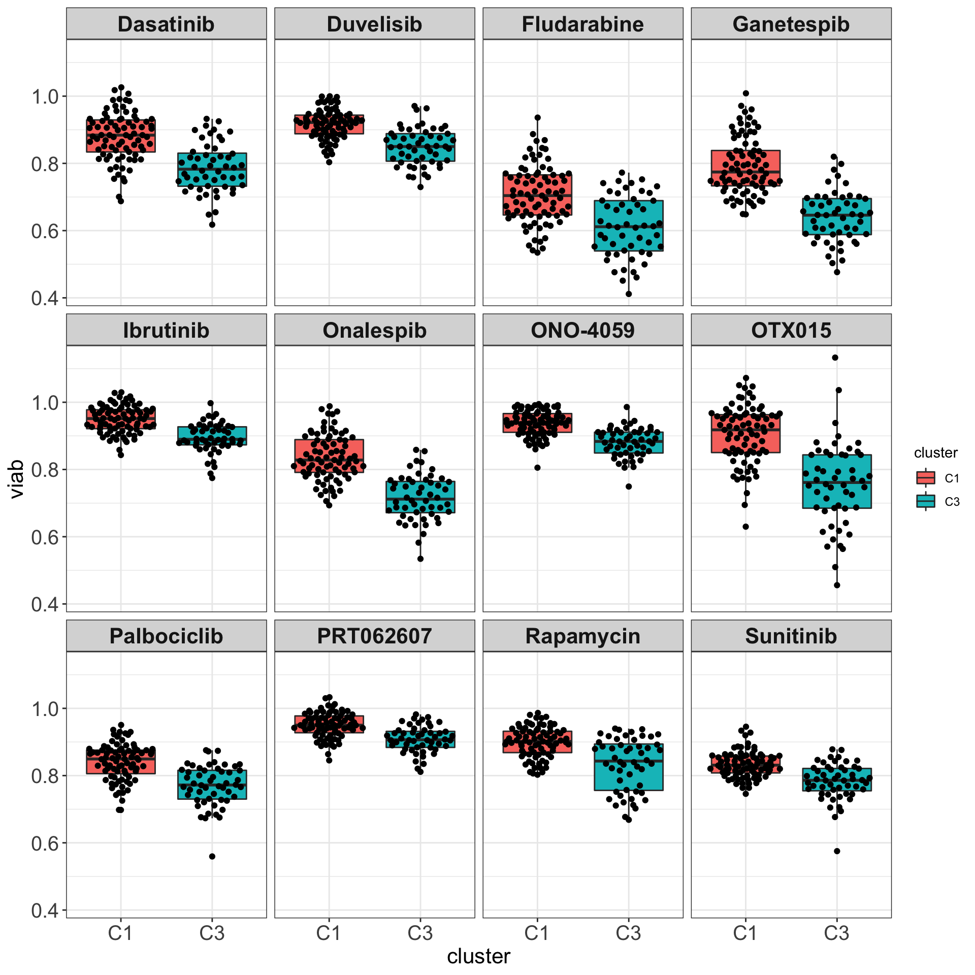
All samples and colored by their IGHV status
drugList <- filter(plotTabVol, drugLabel != "")$Drug
plotTabBox <- filter(testTabAll, Drug %in% drugList, !is.na(IGHV.status))
ggplot(plotTabBox, aes(x=cluster, y = viab)) +
  geom_boxplot(outlier.shape = NA) +
  ggbeeswarm::geom_quasirandom(aes(col= IGHV.status)) +
  scale_color_manual(values = c(M = "#E41A1C", U = "#377EB8")) +
  facet_wrap(~Drug, ncol=4) +
  ylab("Viability (AUC)") + xlab("Clusters") +
  theme_my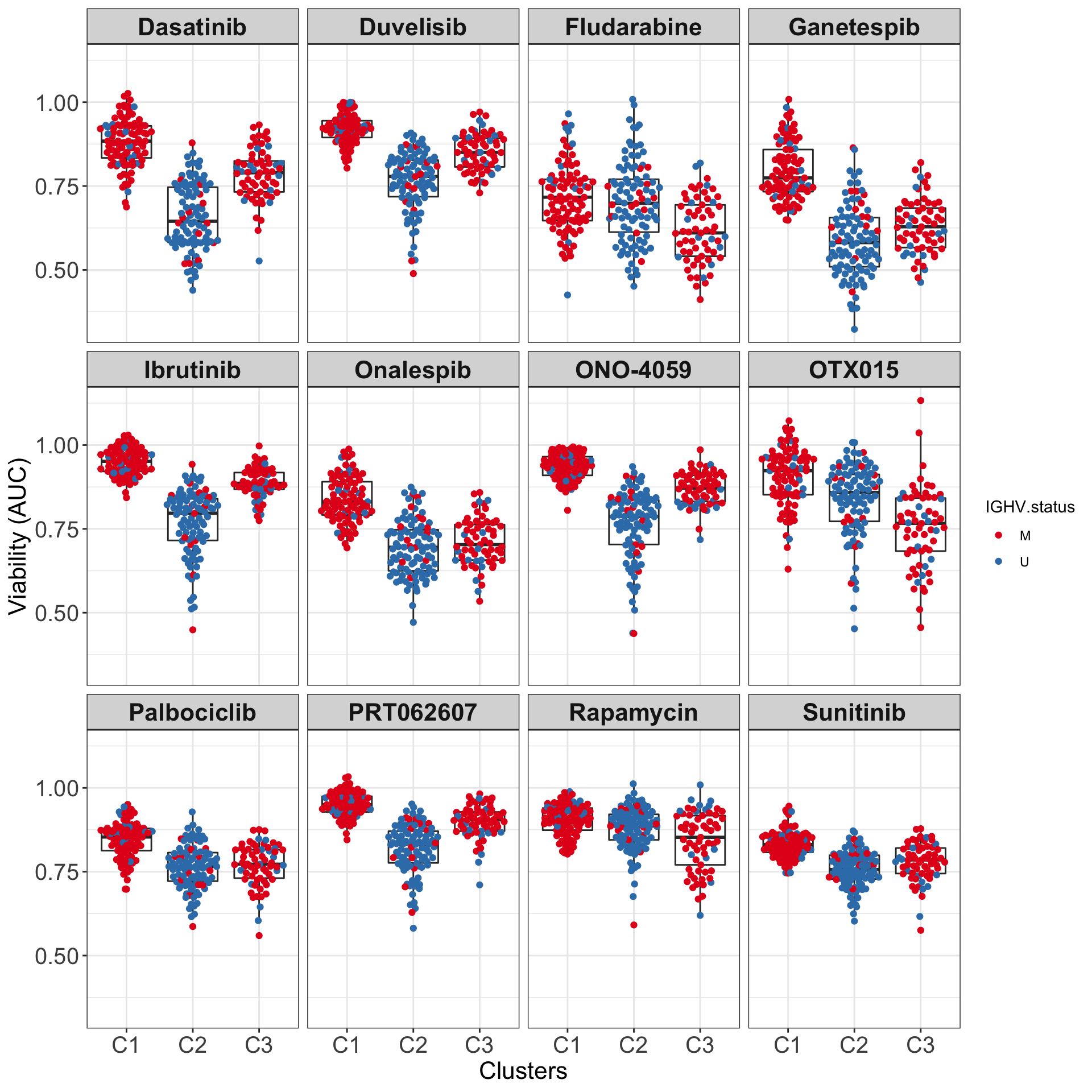
ggsave("boxplot_AUC.png", height = 6, width = 12)It can be seen that for many drugs, the difference between C1 and C3 groups are even larger than between C2 (U-CLL) and C1 or C2 and C3.
Boxplots (C1, C2 and C3) colored by methylation cluster
drugList <- filter(plotTabVol, drugLabel != "")$Drug
plotTabBox <- filter(testTabAll, Drug %in% drugList)
ggplot(plotTabBox, aes(x=cluster, y = viab)) +
geom_boxplot(outlier.shape = NA) +
ggbeeswarm::geom_quasirandom(aes(col= Mclust)) +
facet_wrap(~Drug) +
theme_my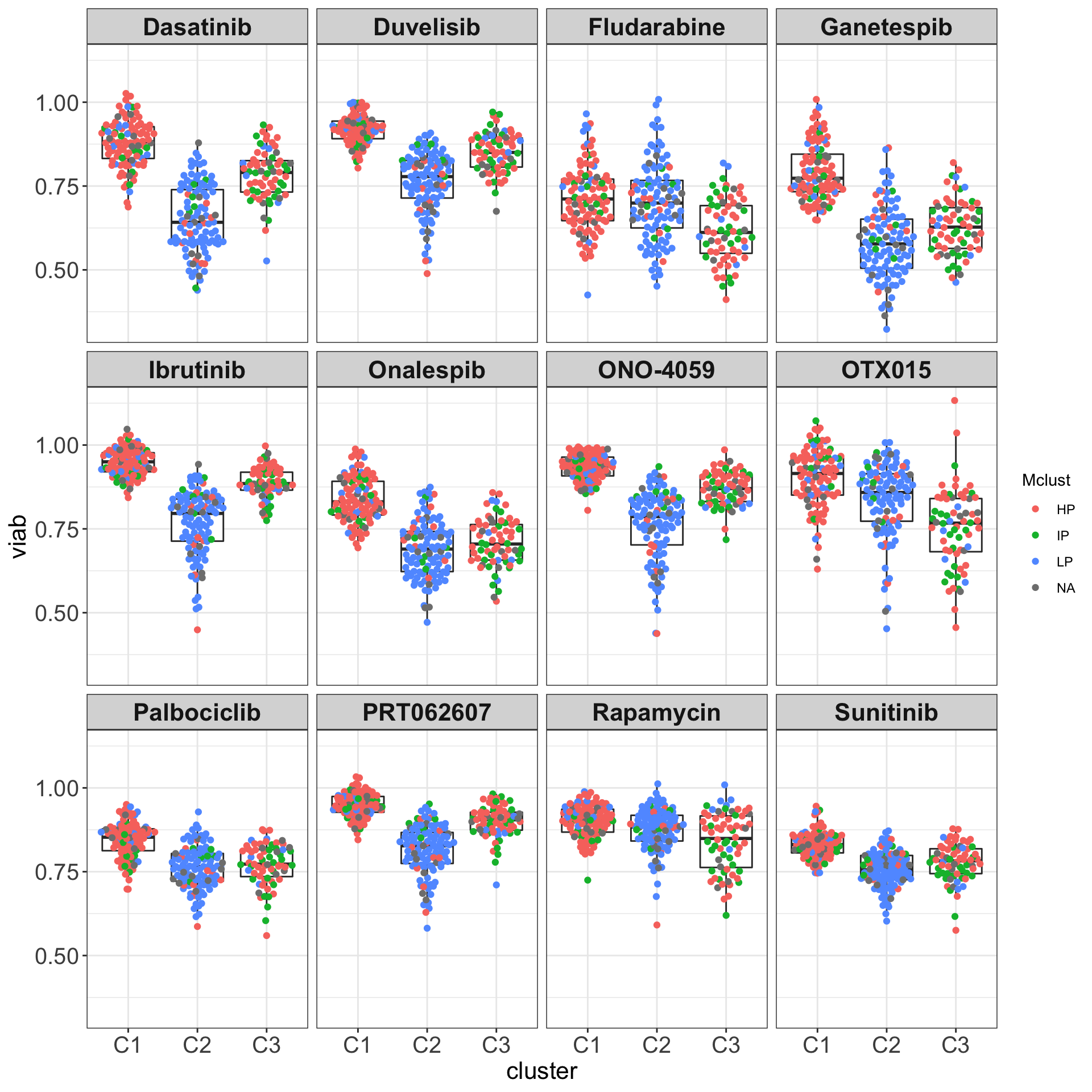 The methylation groups do not explain the difference between C1 and C3 groups.
Dose-response curves
drugList <- filter(plotTabVol, drugLabel != "")$Drug
plotTabCurve <- filter(screenData, Drug %in% drugList) %>%
  left_join(clusterTab) %>% filter(cluster %in% c("C1","C3"))
ggplot(plotTabCurve, aes(x=conc, y = viab, col = cluster, group = sampleID)) +
  #geom_smooth(geom="line", method = "loess", se=FALSE, alpha=0.5, size=0.5) +
  scale_x_log10() +
  geom_line() +
  scale_color_manual(values = c(C1 = "#4DAF4A", C2 = "#984EA3", C3 = "#FF7F00")) +
  facet_wrap(~Drug, ncol=4) +
  theme_my + xlab("concentration") + ylab("viability")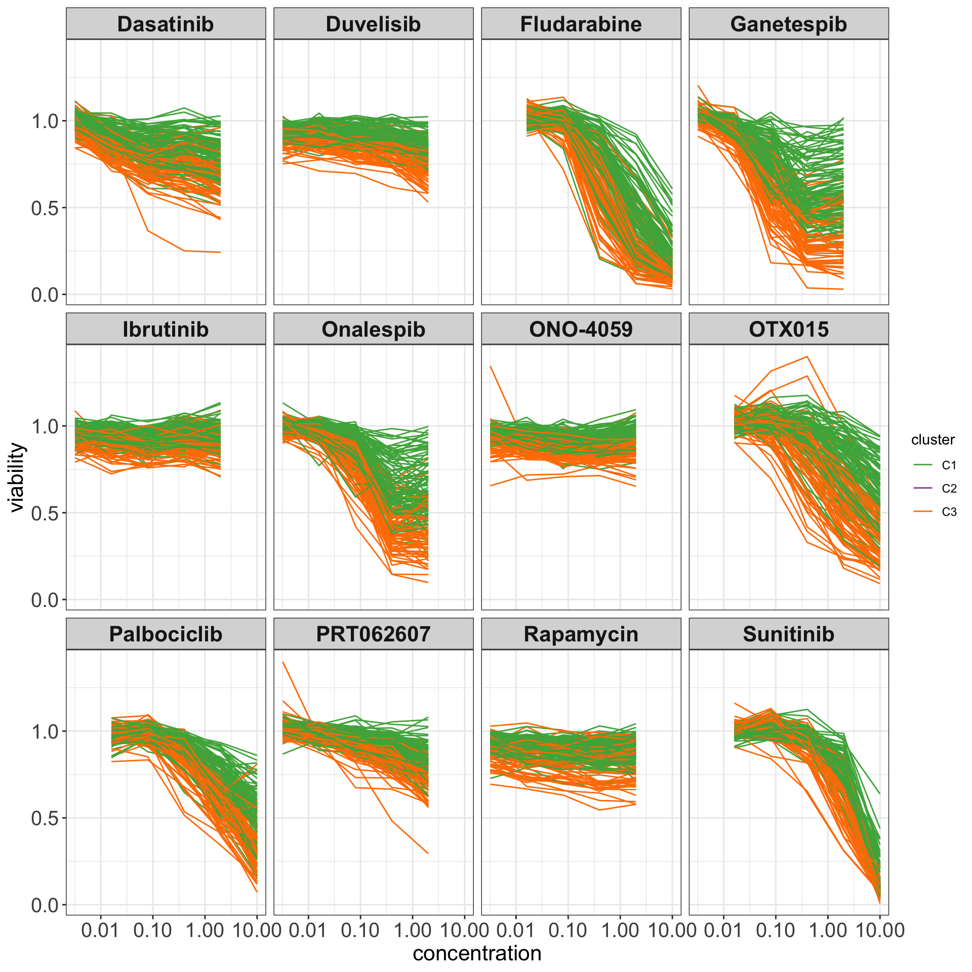
ggsave("dose_curve.png", height = 6, width = 12)General toxicity and group
resTabSig <- filter(resTab, p.adj < 0.1 )
meanViabTab <- filter(screenData,  Drug %in% resTab$Drug) %>%
  group_by(Drug) %>% summarise(meanViab = mean(viab.auc, na.rm=TRUE)) %>%
  mutate(ifSig = ifelse(Drug %in% resTabSig$Drug,"yes","no"))

t.test(meanViab ~ ifSig, meanViabTab)
    Welch Two Sample t-test

data:  meanViab by ifSig
t = 3.1493, df = 54.723, p-value = 0.002651
alternative hypothesis: true difference in means between group no and group yes is not equal to 0
95 percent confidence interval:
 0.0274007 0.1233293
sample estimates:
 mean in group no mean in group yes
         0.961179          0.885814
ggplot(meanViabTab, aes(x=ifSig, y=meanViab)) +
geom_boxplot() + geom_point() +
theme_my +
ylab("mean viability among all samples") + xlab("Associated with C1/C3 clusters")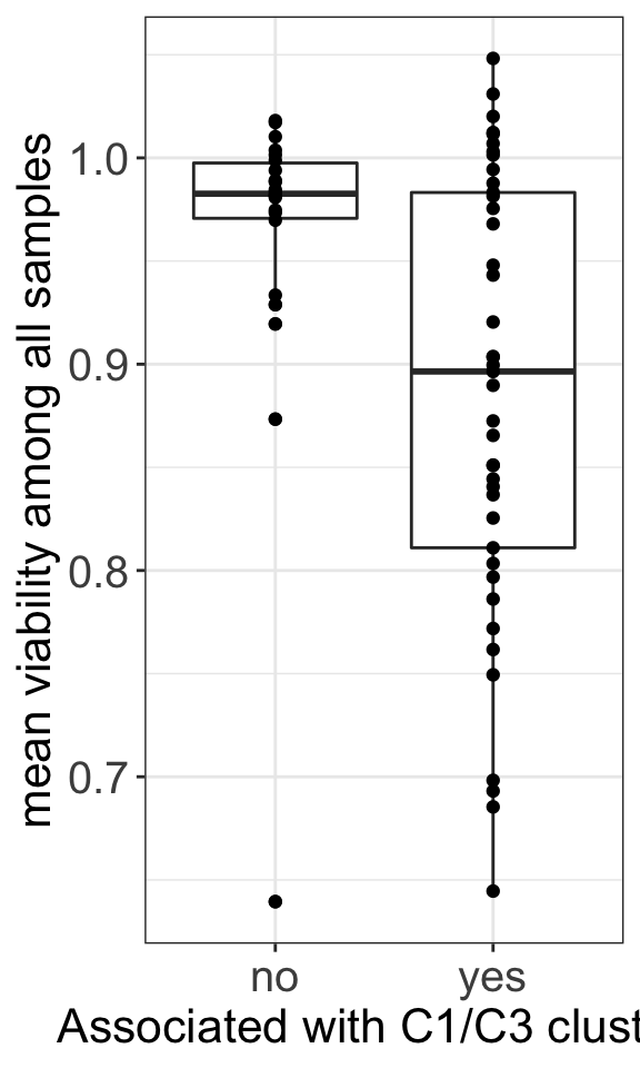
ggsave("toxivity_box.png", width = 5, height = 4)Multi-omics characterization of C1 and C3 groups
In this part, I want to answer the questions that why samples in C1 and C3 groups response differently to those above drugs. In order to explain this, I will look at some of the omics data we have.
Does it correlate with previous identified mTOR group?
All CLLs
drugGroup <- read_csv("~/CLLproject_jlu/data/expressionAnalysis/selNEW.csv") %>%
  dplyr::rename(patID = "...1") %>% select(patID, group) %>%
  mutate(cluster = clusterTab[match(patID, clusterTab$patientID),]$cluster) %>%
  filter(!is.na(cluster))

table(drugGroup$group, drugGroup$cluster)
       C1 C2 C3
  BTK   0 22  2
  MEK   6  7  3
  mTOR  3  2  9
  none 34 15 16
Within M-CLLs
drugGroup <- mutate(drugGroup, IGHV = patMeta[match(patID, patMeta$Patient.ID),]$IGHV.status) %>%
  filter(cluster %in% c("C1","C3"), IGHV %in% "M")
table(drugGroup$group, drugGroup$cluster)
       C1 C3
  BTK   0  1
  MEK   4  2
  mTOR  3  8
  none 31 11
The C1 and C3 groups identified from EMBL2016 screen are not the same as drug sensitivity groups previously identified. Although the C1 group maybe related to the non-responder group. But C3 is not the mTOR group
plotEve <- filter(screenData, Drug %in% c("Everolimus","Rapamycin")) %>%
  group_by(Drug, patientID) %>% summarise(viab = mean(viab.auc)) %>%
  mutate(cluster = clusterTab[match(patientID, clusterTab$patientID),]$cluster,
         IGHV = patMeta[match(patientID, patMeta$Patient.ID),]$IGHV.status) %>%
  filter(cluster %in% c("C1","C3"), IGHV %in% "M")

ggplot(plotEve, aes(x=cluster, y = viab)) +
  geom_boxplot(width=0.3) +
  ggbeeswarm::geom_quasirandom(aes(col = cluster)) +
  scale_color_manual(values = annoCol$cluster) +
  facet_wrap(~Drug) +
  ylab("Viability (AUC)") +
  theme_my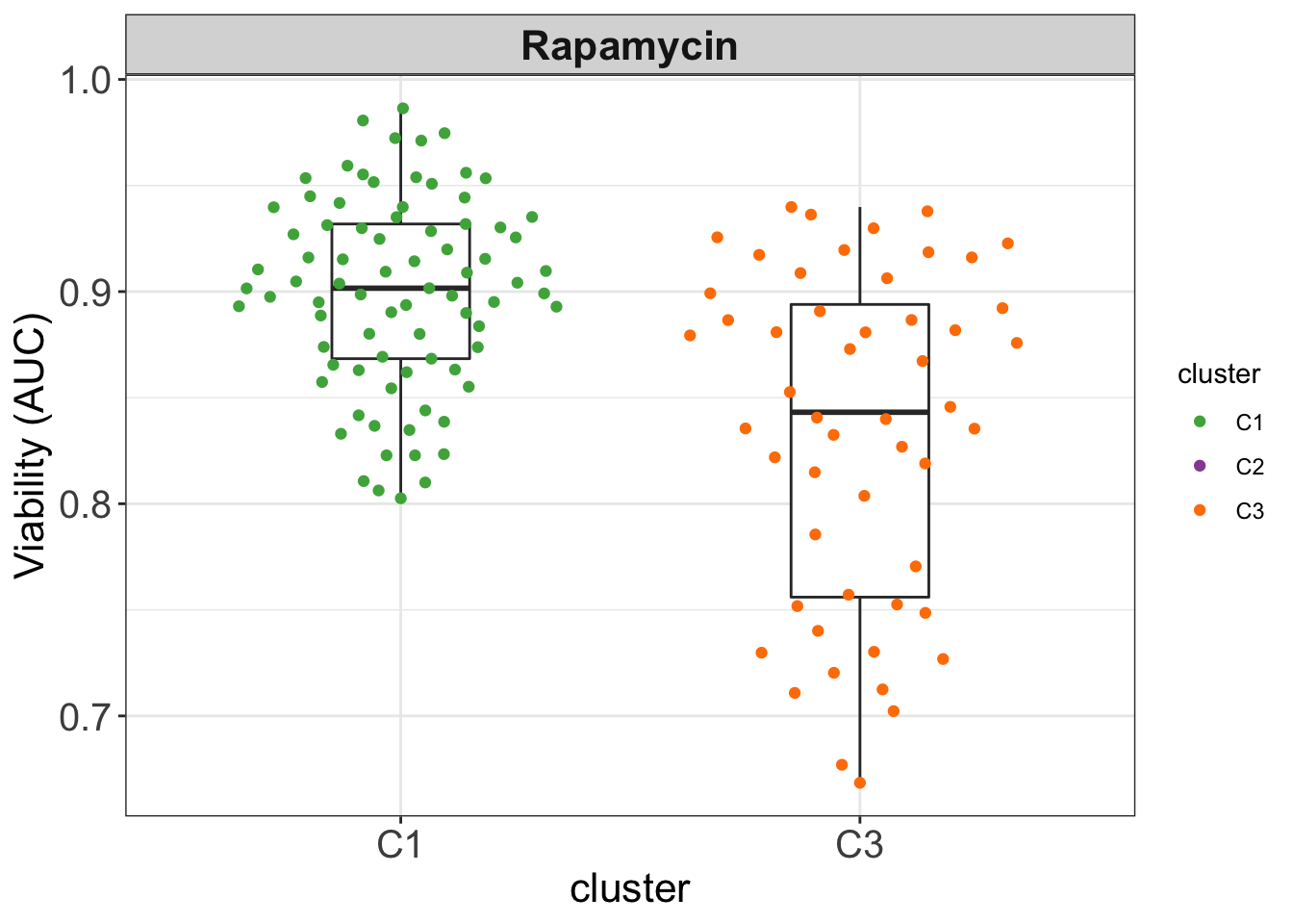
Correlations between genomics/demographics and C1/C3 groups
clusterAnno <- filter(clusterTab, cluster %in% c("C1","C3"), IGHV.status == "M") %>%
  mutate(pretreat = treatmentTab[match(sampleID, treatmentTab$sampleID),]$pretreat)
geneTab <- select(patMeta, Patient.ID, gender, Methylation_Cluster, del10p:U1) %>%
  dplyr::rename(sex = gender)
testTab <- select(clusterAnno, patientID, cluster, pretreat) %>%
  left_join(geneTab, by = c(patientID = "Patient.ID")) %>%
  mutate_all(as.character) %>%
  pivot_longer(!c(patientID, cluster))

sumTab <- group_by(testTab, name) %>%
  summarise(noNA = sum(!is.na(value)), numMut = sum(value %in% c("1","m","HP", "M"))) %>%
  filter(noNA > 40, numMut >=5)

testTab <- filter(testTab, name %in% sumTab$name)
resTab <- group_by(testTab, name) %>% nest() %>%
mutate(m=map(data, ~chisq.test(.$cluster, .$value))) %>%
mutate(res = map(m, broom::tidy)) %>%
unnest(res) %>%
select(name, p.value) %>%
arrange(p.value) %>% ungroup() %>%
mutate(padj = p.adjust(p.value, method = "BH"))
resTab# A tibble: 18 × 3
name p.value padj
<chr> <dbl> <dbl>
1 Methylation_Cluster 0.00714 0.0725
2 SF3B1 0.00805 0.0725
3 TP53 0.0634 0.381
4 HIST1H1E 0.168 0.737
5 pretreat 0.205 0.737
6 ATM 0.335 1
7 trisomy12 0.485 1
8 del5IgH 0.698 1
9 sex 0.719 1
10 del13q 0.957 1
11 del11q 0.959 1
12 gain8q 0.966 1
13 CSMD3 1.00 1
14 NOTCH1 1.00 1
15 del8p 1.00 1
16 del17p 1 1
17 gain18q 1 1
18 IgH_break 1 1 No significant associations can be identified, indicating the C1/C3 group is not driven by genomic, demographic or treatment. It can potentially be a new functional group
Whether it correlates with CLL-PD?
load("~/CLLproject_jlu/analysis/CLLsubgroup/facTab_CPSatLeast3New.RData")
testTab <- clusterAnno %>%
  mutate(CLLPD = facTab[match(patientID, facTab$patID),]$factor)

t.test(CLLPD ~ cluster, testTab, var.equal=TRUE)
    Two Sample t-test

data:  CLLPD by cluster
t = -2.9444, df = 96, p-value = 0.004059
alternative hypothesis: true difference in means between group C1 and group C3 is not equal to 0
95 percent confidence interval:
 -0.9339167 -0.1817678
sample estimates:
mean in group C1 mean in group C3
      -0.4156659        0.1421763
ggplot(testTab, aes(x=cluster, y=CLLPD)) +
geom_boxplot(outlier.shape = NA, width=0.3) +
ggbeeswarm::geom_quasirandom(aes(col = cluster)) +
scale_color_manual(values = annoCol$cluster) +
ylab("CLL-PD") +
theme_my + theme(legend.position = "none")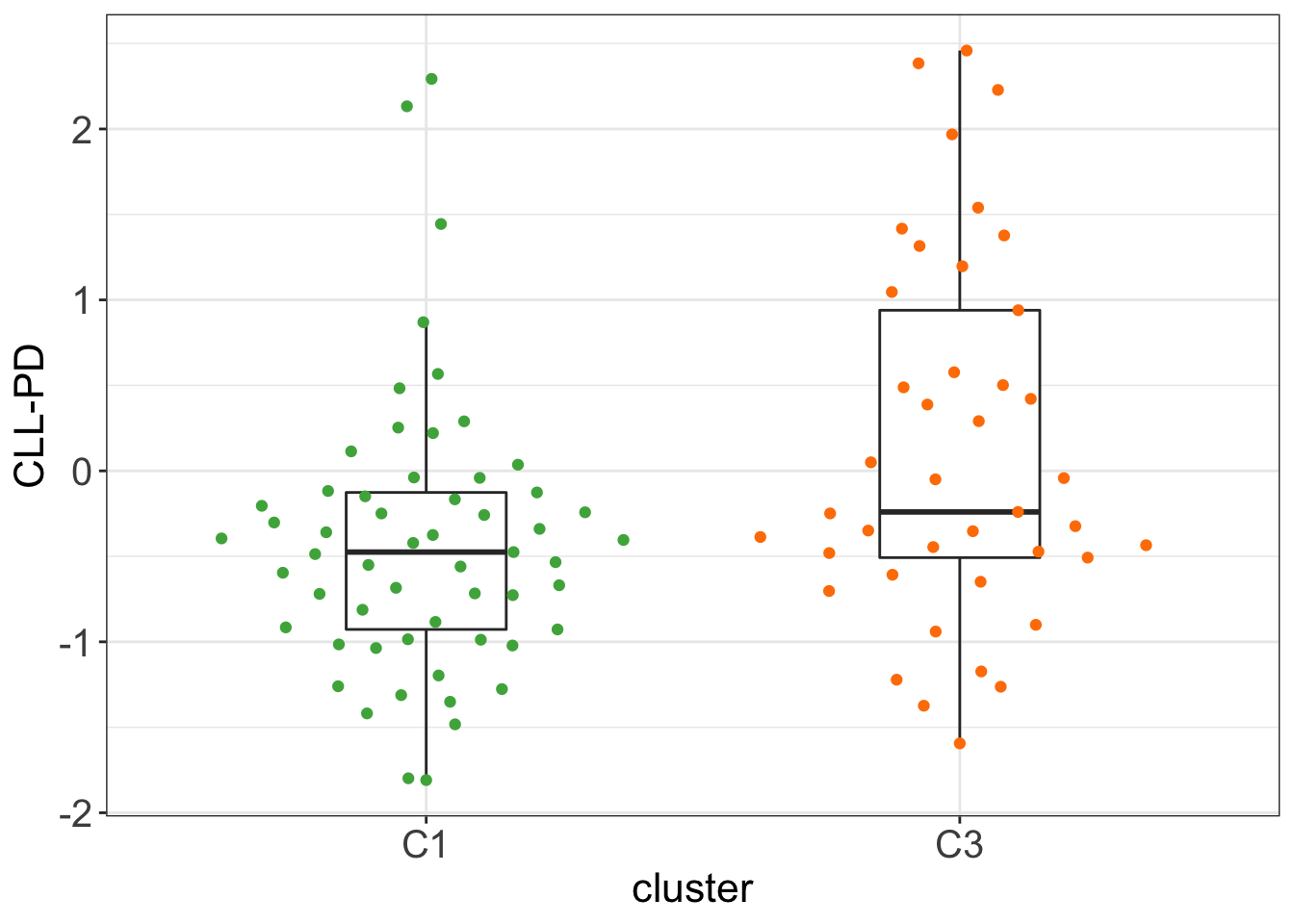 There is a significant correlations between CLL-PD and C1/C3 group, but not very strong.
Baseline ATP levels after 48 hours
Baseline ATP is the ATP level in the control wells after 48 hours of culture. It can be regarded as a baseline viability of the cells.
load("~/CLLproject_jlu/var/CPS1000_mainAnalysis.RData")
basalATP <- pheno1000_main %>% filter(Drug == "DMSO", !edge) %>%
  group_by(patientID) %>% summarise(ATPcount = median(val, na.rm=TRUE))
testTab <- clusterAnno %>%
left_join(basalATP, by = c(patientID = "patientID"))
t.test(log(ATPcount) ~ cluster, testTab, var.equal=TRUE)
    Two Sample t-test

data:  log(ATPcount) by cluster
t = 5.8947, df = 131, p-value = 3.004e-08
alternative hypothesis: true difference in means between group C1 and group C3 is not equal to 0
95 percent confidence interval:
 0.2730595 0.5489072
sample estimates:
mean in group C1 mean in group C3
        14.58283         14.17185
ggplot(testTab, aes(x=cluster, y=log(ATPcount))) +
geom_boxplot(outlier.shape = NA, width=0.3) +
ggbeeswarm::geom_quasirandom(aes(col = cluster)) +
scale_color_manual(values = annoCol$cluster) +
ylab("baseline ATP") +
theme_my + theme(legend.position = "none")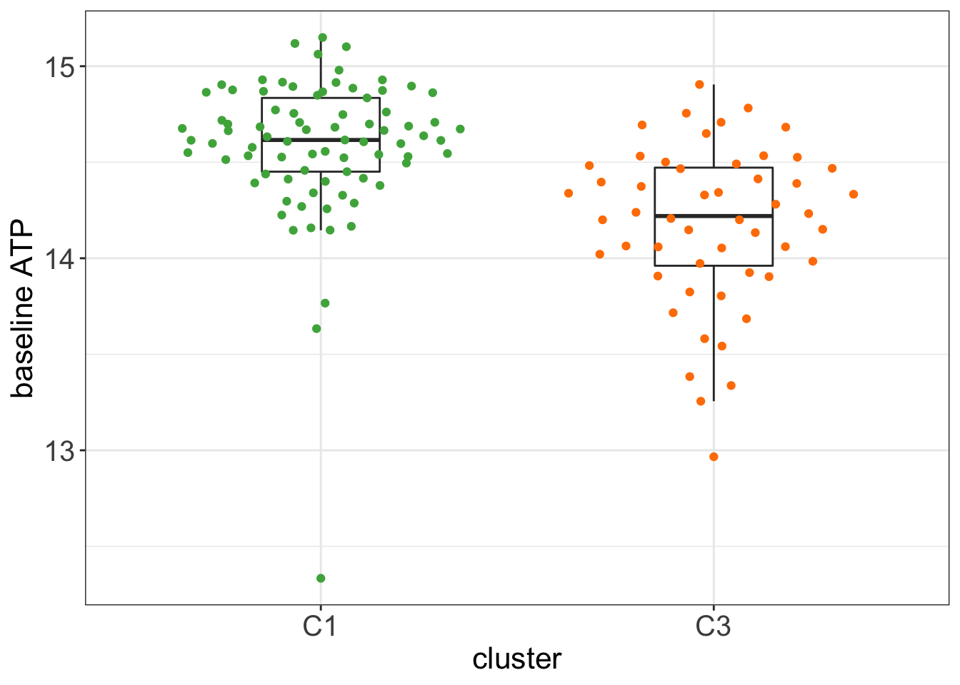 There is a pretty strong correlation between C1/C3 group and baseline ATP.
Does CLL-PD correlate basal ATP?
testTab <- testTab %>%
  mutate(CLLPD = facTab[match(patientID, facTab$patID),]$factor)

cor.test(~CLLPD + log(ATPcount), testTab)
    Pearson's product-moment correlation

data:  CLLPD and log(ATPcount)
t = -0.92622, df = 96, p-value = 0.3567
alternative hypothesis: true correlation is not equal to 0
95 percent confidence interval:
 -0.2871703  0.1062936
sample estimates:
        cor
-0.09411205
ggplot(testTab, aes(x=CLLPD, y= log10(ATPcount))) +
geom_point() + geom_smooth(method ="lm") +
theme_my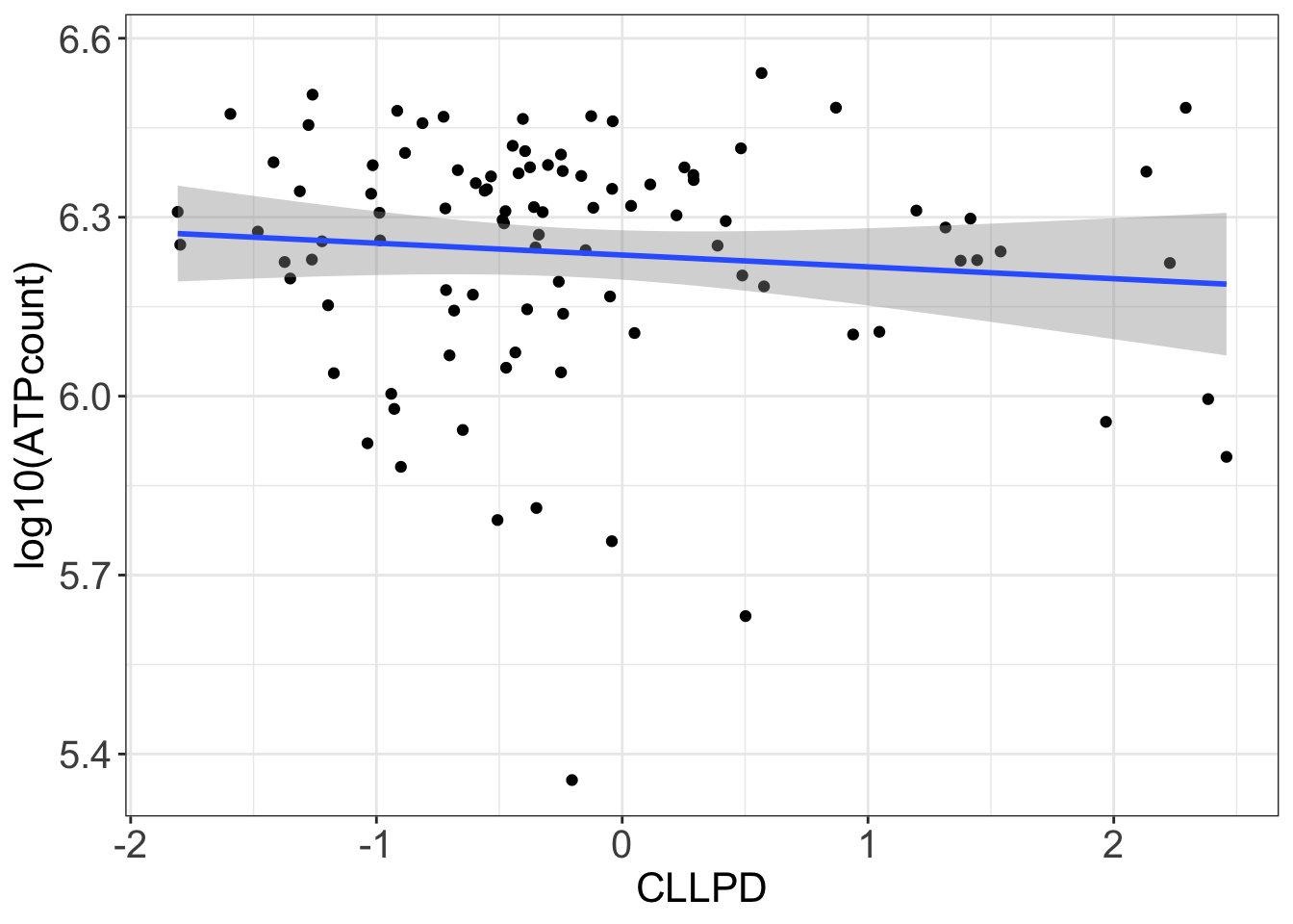 No.
No.
Multi-variate model to explain C1/C2
testTab <- mutate(testTab, cluster = factor(cluster)) %>% mutate(cluster = as.integer(cluster))
car::Anova(lm(cluster ~ log10(ATPcount) + CLLPD, testTab))
Anova Table (Type II tests)
Response: cluster
Sum Sq Df F value Pr(>F)
log10(ATPcount) 4.8416 1 27.0079 1.157e-06 ***
CLLPD 1.4211 1 7.9272 0.005921 **
Residuals 17.0302 95
---
Signif. codes: 0 '***' 0.001 '**' 0.01 '*' 0.05 '.' 0.1 ' ' 1Both CLL-PD and baseline ATP explain C1/C3 group separation.
Transcriptomic characterization.
Differential gene expression between C1 and C3 groups
load("../../var/ddsrna_180717.RData")
dds$cluster <- factor(clusterAnno[match(dds$PatID, clusterAnno$patientID),]$cluster)
dds$CLLPD <- facTab[match(dds$PatID, facTab$patID),]$factor
dds$IGHV <- factor(patMeta[match(dds$PatID, patMeta$Patient.ID),]$IGHV.status)
ddsSub <- dds[,!is.na(dds$cluster)]
ddsSub <- ddsSub[rowMedians(counts(ddsSub, normalized = TRUE)) > 10,]
ddsSub <- ddsSub[rowData(ddsSub)$biotype %in% "protein_coding",]
ddsSub <- ddsSub[!rowData(ddsSub)$symbol %in% c("", NA)]library(DESeq2)
design(ddsSub) <- ~cluster
deRes <- DESeq(ddsSub)Table of differentially expressed genes (10% FDR)
resTab <- results(deRes, tidy = TRUE, name = "cluster_C3_vs_C1") %>%
  mutate(symbol = rowData(ddsSub[row,])$symbol) %>%
  arrange(pvalue)

resTab.sig <- filter(resTab, padj < 0.1) %>%
  mutate(symbol = factor(symbol, levels = symbol))
DT::datatable(resTab.sig %>% select(symbol, row, stat, pvalue, padj) %>%
                mutate_if(is.numeric, formatC, digits=2))
P-value histogram
hist(resTab$pvalue)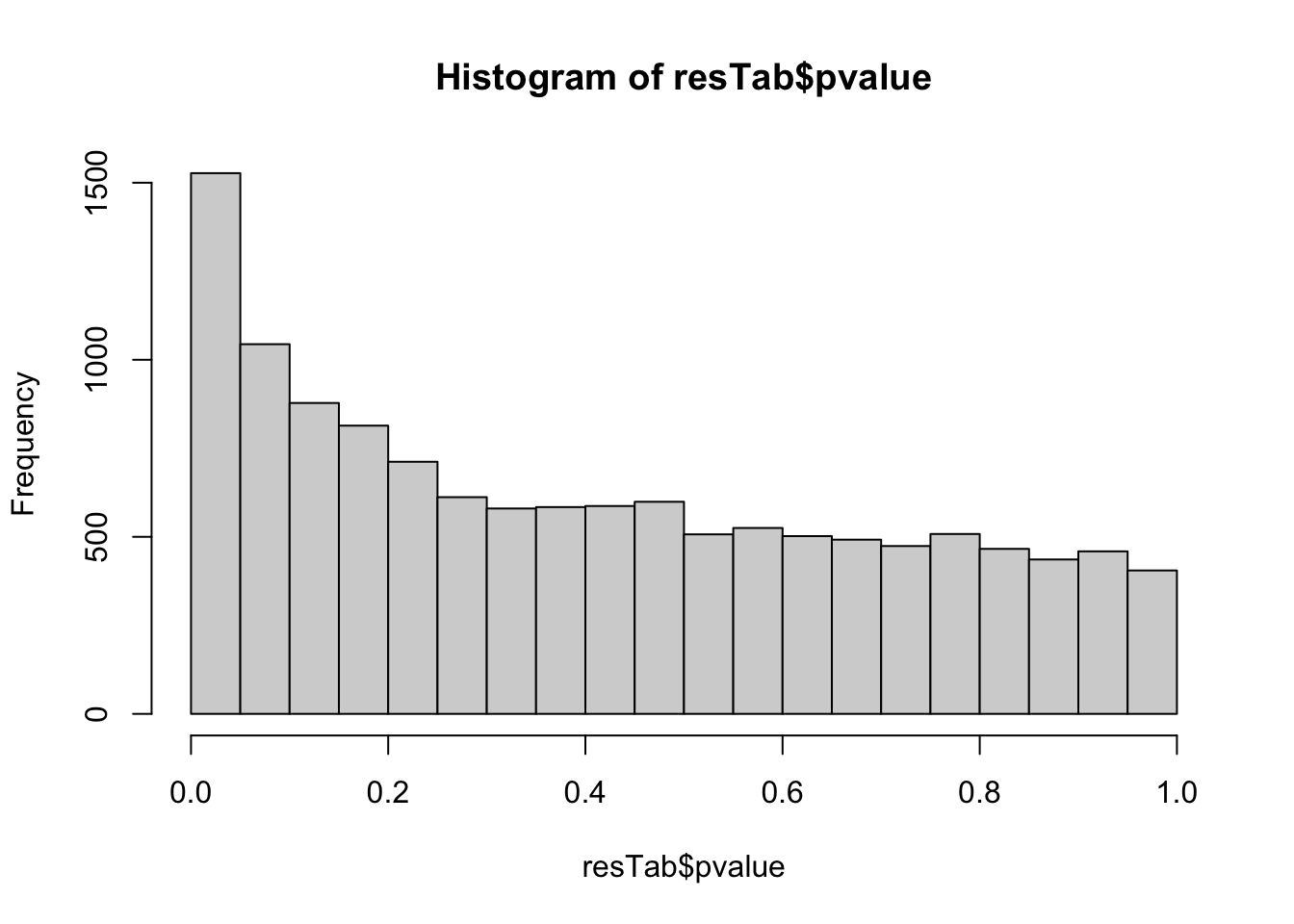
Boxplots of top 9 candidates based on p-value
plotTab <- counts(ddsSub, normalized = TRUE)[resTab.sig$row[1:9],] %>%
  as_tibble(rownames = "id") %>% pivot_longer(-id) %>%
  mutate(cluster = clusterAnno[match(name, clusterAnno$patientID),]$cluster) %>%
  left_join(resTab.sig, by = c(id = "row"))

ggplot(plotTab, aes(x=cluster, y=log10(value))) +
  geom_boxplot(outlier.shape = NA, width=0.3) +
  ggbeeswarm::geom_quasirandom(aes(col=cluster)) +
  facet_wrap(~symbol, scale ="free") +
  scale_color_manual(values = annoCol$cluster) +
  ylab("RNAseq count") +
  theme_my + theme(legend.position = "none")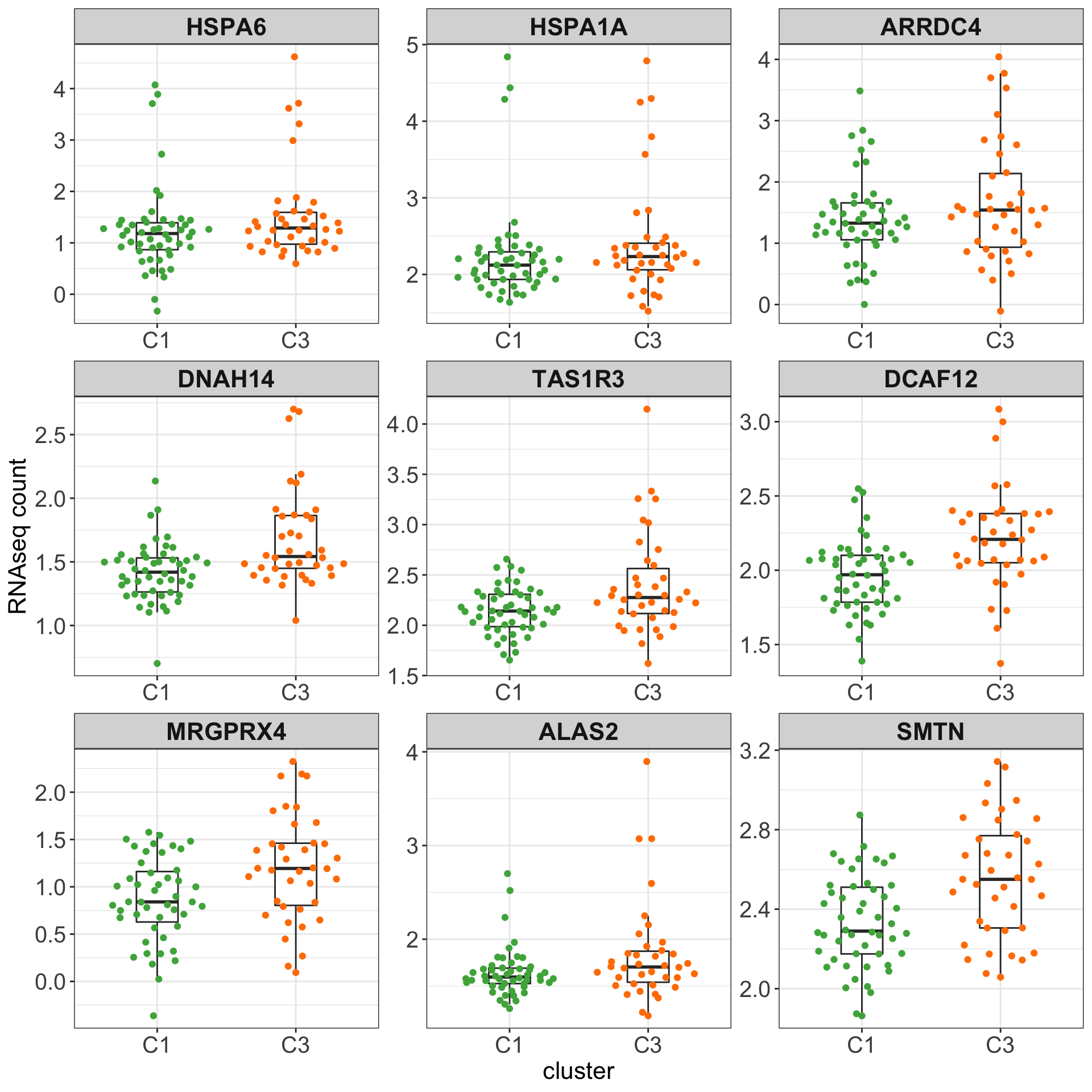
Pathway enrichment analysis
exprMat <- counts(ddsSub)
exprMat <- limma::voom(exprMat, lib.size = ddsSub$sizeFactor)$E
designMat <- model.matrix(~ddsSub$cluster)
Hallmark gene sets
(Raw p values < 0.05, no sets passed 10% FDR)
gmts <- list(H = "~/CLLproject_jlu/data/commonFiles/h.all.v6.2.symbols.gmt",
             KEGG = "~/CLLproject_jlu/data/commonFiles/c2.cp.kegg.v5.1.symbols.gmt")
enHallmark <- jyluMisc::runCamera(exprMat, designMat, gmts$H, id = rowData(ddsSub)$symbol,ifFDR = FALSE, pCut =0.05, plotTitle = "Cancer Hallmarks")
enHallmark$enrichPlot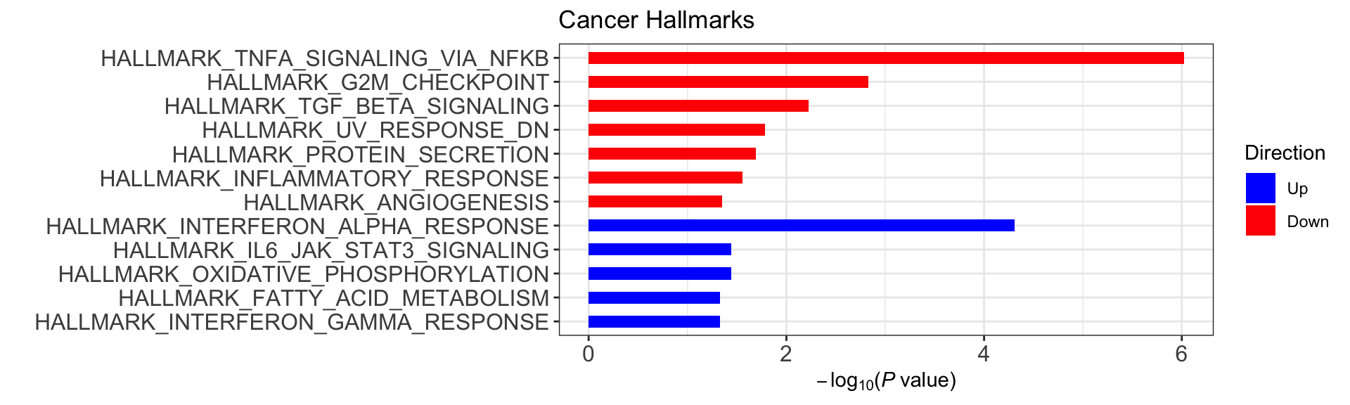
KEGG gene set
(Raw p values < 0.05, no sets passed 10% FDR)
gmts <- list(H = "~/CLLproject_jlu/data/commonFiles/h.all.v6.2.symbols.gmt",
             KEGG = "~/CLLproject_jlu/data/commonFiles/c2.cp.kegg.v5.1.symbols.gmt")
enHallmark <- jyluMisc::runCamera(exprMat, designMat, gmts$KEGG, id = rowData(ddsSub)$symbol,ifFDR = FALSE, pCut =0.01, plotTitle = "KEGG gene sets")
enHallmark$enrichPlot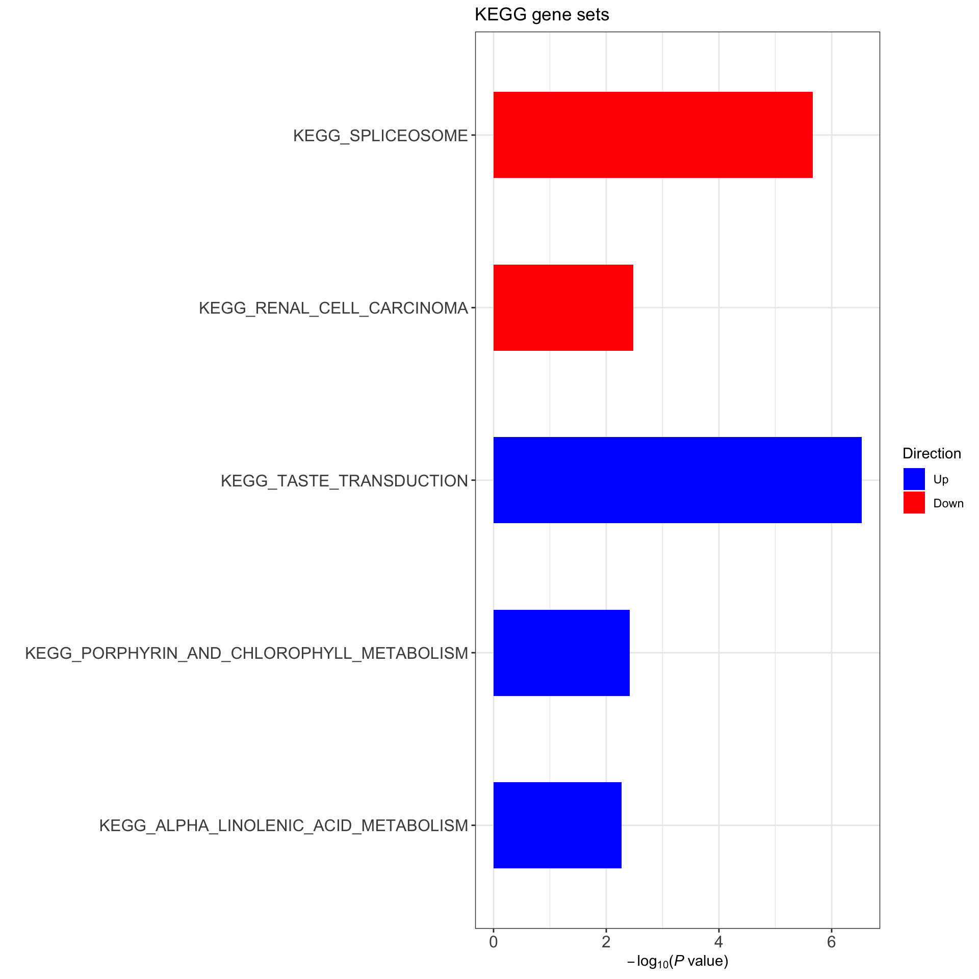
Differential expression at protein levels
load("../../var/proteomic_LUMOS_batch13.RData")
protCLL$patID <- colnames(protCLL)
protCLL$cluster <- factor(clusterAnno[match(protCLL$patID, clusterAnno$patientID),]$cluster)
protCLL$CLLPD <- facTab[match(protCLL$patID, facTab$patID),]$factor
protCLL$IGHV <- factor(patMeta[match(protCLL$patID, patMeta$Patient.ID),]$IGHV.status)
protSub <- protCLL[,!is.na(protCLL$cluster)]

table(protSub$cluster)
C1 C3
19 18
protSub <- protSub[,!is.na(protSub$cluster)]Differential expression
library(proDA)
designMat <- data.frame(row.names = protSub$patID,
                         cluster = protSub$cluster,
                         batch = protSub$batch)

protMat <- assays(protSub)[["count"]]

fit <- proDA(protMat, design = ~ .,
             col_data = designMat)

resTab <- test_diff(fit, "clusterC3") %>%
  dplyr::rename(id = name, logFC = diff, t=t_statistic,
                pvalue = pval, padj = adj_pval) %>%
  mutate(symbol = rowData(protCLL[id,])$hgnc_symbol) %>%
  select(symbol, id, logFC, t, pvalue, padj, n_obs) %>%
  arrange(pvalue) %>%
  as_tibble()
Tables of candiates with P value < 0.01
(none passed 10% FDR)
resTab.sig <- filter(resTab, pvalue < 0.01) %>%
  mutate(symbol = factor(symbol, levels = symbol))
DT::datatable(resTab.sig %>% select(symbol, logFC, pvalue, padj) %>%
                mutate_if(is.numeric, formatC, digits=2))
P-value histogram
hist(resTab$pvalue)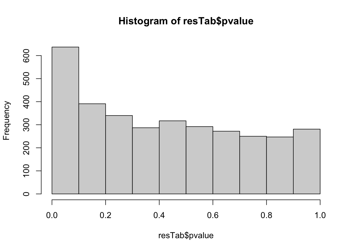
Boxplots of top 9 candidates
plotTab <- assays(protSub)[["log2Norm_combat"]][resTab.sig$id[1:9],] %>%
  as_tibble(rownames = "id") %>% pivot_longer(-id) %>%
  mutate(cluster = clusterAnno[match(name, clusterAnno$patientID),]$cluster) %>%
  left_join(resTab.sig, by = "id")

ggplot(plotTab, aes(x=cluster, y=log10(value))) +
  geom_boxplot(outlier.shape = NA, width=0.3) +
  ggbeeswarm::geom_quasirandom(aes(col = cluster)) +
  scale_color_manual(values = annoCol$cluster) +
  facet_wrap(~symbol, scale ="free") +
  theme_my + theme(legend.position = "none")
Association with BH3 profiling data
load("../../BH3profiling/output/dynamicBH3.RData")
dataBH3 <- dynamicBH3 %>% filter(drug == "DMSO", peptide != "DMSO") %>%
  distinct(patID, peptide, .keep_all = TRUE) %>%
  mutate(feature = peptide, value = AUC, concIndex =1) %>%
  mutate(cluster = clusterAnno[match(patID, clusterAnno$patientID),]$cluster) %>%
  filter(!is.na(cluster))

tRes <- group_by(dataBH3, feature) %>% nest() %>%
  mutate(m = map(data, ~t.test(value ~ cluster,., var.equal=TRUE))) %>%
  mutate(res = map(m, broom::tidy)) %>%
  unnest(res) %>%
  arrange(p.value)

head(tRes)
# A tibble: 6 × 13
# Groups: feature [6]
feature data m estimate estimate1 estimate2 statistic p.value
<chr> <list> <list> <dbl> <dbl> <dbl> <dbl> <dbl>
1 MS1 <tibble> <htest> -12.8 31.5 44.3 -2.05 0.0492
2 BIM <tibble> <htest> -8.92 51.3 60.2 -1.90 0.0672
3 FS1 <tibble> <htest> -7.26 20.3 27.6 -1.64 0.112
4 A133 <tibble> <htest> -6.38 35.3 41.7 -1.20 0.239
5 HRKy <tibble> <htest> 1.30 3.54 2.23 0.801 0.430
6 PUMA <tibble> <htest> -3.31 51.6 54.9 -0.545 0.590
# … with 5 more variables: parameter <dbl>, conf.low <dbl>, conf.high <dbl>,
# method <chr>, alternative <chr>plotTab <- dataBH3 %>% filter(feature %in% c("FS1","MS1", "BIM"))
ggplot(plotTab, aes(x=cluster ,y = value)) +
geom_boxplot(width=0.5) +
geom_point(aes(col = cluster)) +
scale_color_manual(values = annoCol$cluster) +
facet_wrap(~feature) +
ylab("mitochondrial priming") + xlab("") +
theme_my + theme(legend.position = "none")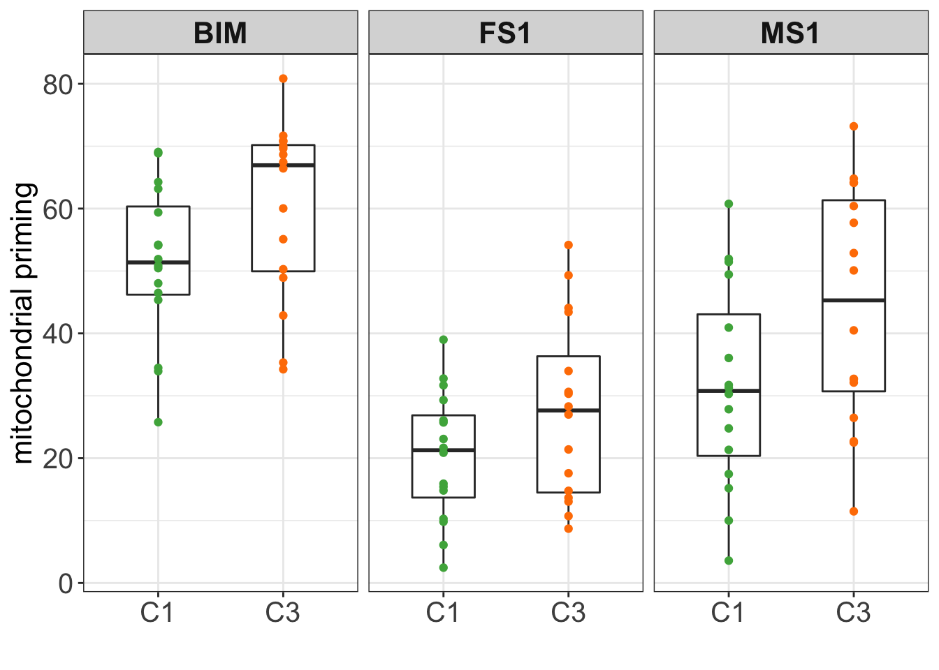
Association with clinical outcomes (TTT and OS)
(Only M-CLL samples clustered as C1 and C3 groups are included)
load("../../var/survival_190516.RData")
testTab <- clusterAnno %>% left_join(survT, by = "sampleID")
Function for cox regression
com <- function(response, time, endpoint, scale =FALSE) {

  if (scale) {
    #calculate z-score
    response <- (response - mean(response, na.rm = TRUE))/sd(response, na.rm=TRUE)
  }
  surv <- coxph(Surv(time, endpoint) ~ response)


  tibble(p = summary(surv)[[7]][,5],
         HR = summary(surv)[[7]][,2],
         lower = summary(surv)[[8]][,3],
         higher = summary(surv)[[8]][,4])
}
Cox regression results
TTT
com(factor(testTab$cluster), testTab$TTT, testTab$treatedAfter)# A tibble: 1 × 4
p HR lower higher
<dbl> <dbl> <dbl> <dbl>
1 0.317 1.44 0.703 2.96OS
com(factor(testTab$cluster), testTab$OS, testTab$died)# A tibble: 1 × 4
p HR lower higher
<dbl> <dbl> <dbl> <dbl>
1 0.365 2.29 0.382 13.7Cox regression results in only un-treated samples
TTT
testTab.untreated <- filter(testTab, pretreat %in% 0)
com(factor(testTab.untreated$cluster), testTab.untreated$TTT, testTab.untreated$treatedAfter)
# A tibble: 1 × 4
p HR lower higher
<dbl> <dbl> <dbl> <dbl>
1 0.861 1.09 0.427 2.77OS
com(factor(testTab.untreated$cluster), testTab.untreated$OS, testTab.untreated$died)# A tibble: 1 × 4
p HR lower higher
<dbl> <dbl> <dbl> <dbl>
1 0.269 2.75 0.458 16.4Cox regression results in only pre-treated samples
TTT
testTab.treated <- filter(testTab, pretreat %in% 1)
com(factor(testTab.treated$cluster), testTab.treated$TTT, testTab.treated$treatedAfter)
# A tibble: 1 × 4
p HR lower higher
<dbl> <dbl> <dbl> <dbl>
1 0.953 0.963 0.270 3.44OS
com(factor(testTab.treated$cluster), testTab.treated$OS, testTab.treated$died)# A tibble: 1 × 4
p HR lower higher
<dbl> <dbl> <dbl> <dbl>
1 NA NA NA NAKaplan-Meier plots
Function for KM plot
formatNum <- function(i, limit = 0.01, digits =1, format="e") {
  r <- sapply(i, function(n) {
    if (n < limit) {
      formatC(n, digits = digits, format = format)
    } else {
      format(n, digits = digits)
    }
  })
  return(r)
}

theme_half <- ggplot2::theme_bw() + ggplot2::theme(axis.text = ggplot2::element_text(size=15),
                                 axis.title = ggplot2::element_text(size=16),
                                 axis.line = ggplot2::element_line(size=0.8),
                                 panel.border = ggplot2::element_blank(),
                                 axis.ticks = ggplot2::element_line(size=1.5),
                                 plot.title = ggplot2::element_text(size = 16, hjust =0.5, face="bold"),
                                 panel.grid.major = ggplot2::element_blank(),
                                 panel.grid.minor = ggplot2::element_blank())

km <- function(response, time, endpoint, titlePlot = "KM plot", pval = NULL,
               stat = "median", maxTime =NULL, showP = TRUE, showTable = FALSE,
               ylab = "Fraction", xlab = "Time (years)",
               table_ratio = c(0.7,0.3), yLabelAdjust = 0) {

  colList <- c("#BC3C29FF","#0072B5FF","#E18727FF","#20854EFF","#7876B1FF","#6F99ADFF","#FFDC91FF","#EE4C97FF")

  #function for km plot
  survS <- tibble(time = time,
                  endpoint = endpoint)

  if (!is.null(maxTime))
    survS <- mutate(survS, endpoint = ifelse(time > maxTime, FALSE, endpoint),
                    time = ifelse(time > maxTime, maxTime, time))

  if (stat == "maxstat") {
    ms <- maxstat.test(Surv(time, endpoint)  ~ response,
                       data = survS,
                       smethod = "LogRank",
                       minprop = 0.2,
                       maxprop = 0.8,
                       alpha = NULL)

    survS$group <- factor(ifelse(response >= ms$estimate, "high", "low"))
    p <- com(survS$group, survS$time, survS$endpoint)$p

  } else if (stat == "median") {
    med <- median(response, na.rm = TRUE)
    survS$group <- factor(ifelse(response >= med, "high", "low"))
    p <- com(survS$group, survS$time, survS$endpoint)$p

  } else if (stat == "binary") {
    survS$group <- factor(response)
    if (nlevels(survS$group) > 2) {
      sdf <- survdiff(Surv(survS$time,survS$endpoint) ~ survS$group)
      p <- 1 - pchisq(sdf$chisq, length(sdf$n) - 1)
    } else {
      p <- com(survS$group, survS$time, survS$endpoint)$p
    }
  }

  if (is.null(pval)) {
    if(p< 1e-16) {
      pAnno <- bquote(italic("P")~"< 1e-16")
    } else {
      pval <- formatNum(p, digits = 1)
      pAnno <- bquote(italic("P")~"="~.(pval))
    }

  } else {
     pval <- formatNum(pval, digits = 1)
     pAnno <- bquote(italic("P")~"="~.(pval))
  }

  if (!showP) pAnno <- ""

  colListNew <- colList[-4] #remove green
  colorPal <- colListNew[1:length(unique(survS$group))]
  p <- ggsurvplot(survfit(Surv(time, endpoint) ~ group, data = survS),
                  data = survS, pval = FALSE,  conf.int = FALSE, palette = colorPal,
                  legend = ifelse(showTable, "none","top"),
                  ylab = "Fraction", xlab = "Time (years)", title = titlePlot,
                  pval.coord = c(0,0.1), risk.table = showTable, legend.labs = sort(unique(survS$group)),
                  ggtheme = theme_half + theme(plot.title = element_text(hjust =0.5),
                                               panel.border = element_blank(),
                                               axis.title.y = element_text(vjust =yLabelAdjust)))
  if (!showTable) {
    p <- p$plot + annotate("text",label=pAnno, x = 0.1, y=0.1, hjust =0, size =5)
    return(p)
  } else {
    #construct a gtable
    pp <- p$plot + annotate("text",label=pAnno, x = 0.1, y=0.1, hjust =0, size=5)
    pt <- p$table + ylab("") + xlab("") + theme(plot.title = element_text(hjust=0, size =10))
    p <- plot_grid(pp,pt, rel_heights = table_ratio, nrow =2, align = "v")
    return(p)
  }
}
TTT
km(testTab$cluster, testTab$TTT, testTab$treatedAfter, "cluster VS TTT", stat = "binary", showTable = TRUE)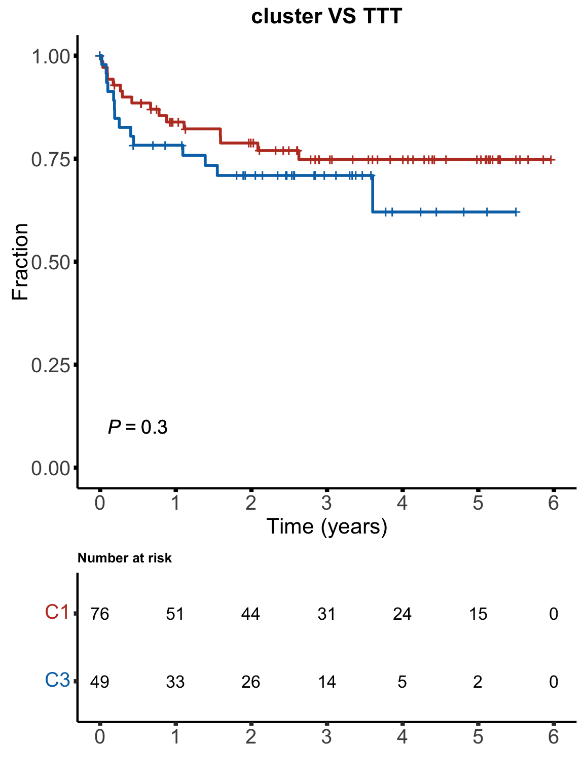
OS
km(testTab$cluster, testTab$OS, testTab$died, "cluster VS OS", stat = "binary", showTable = TRUE)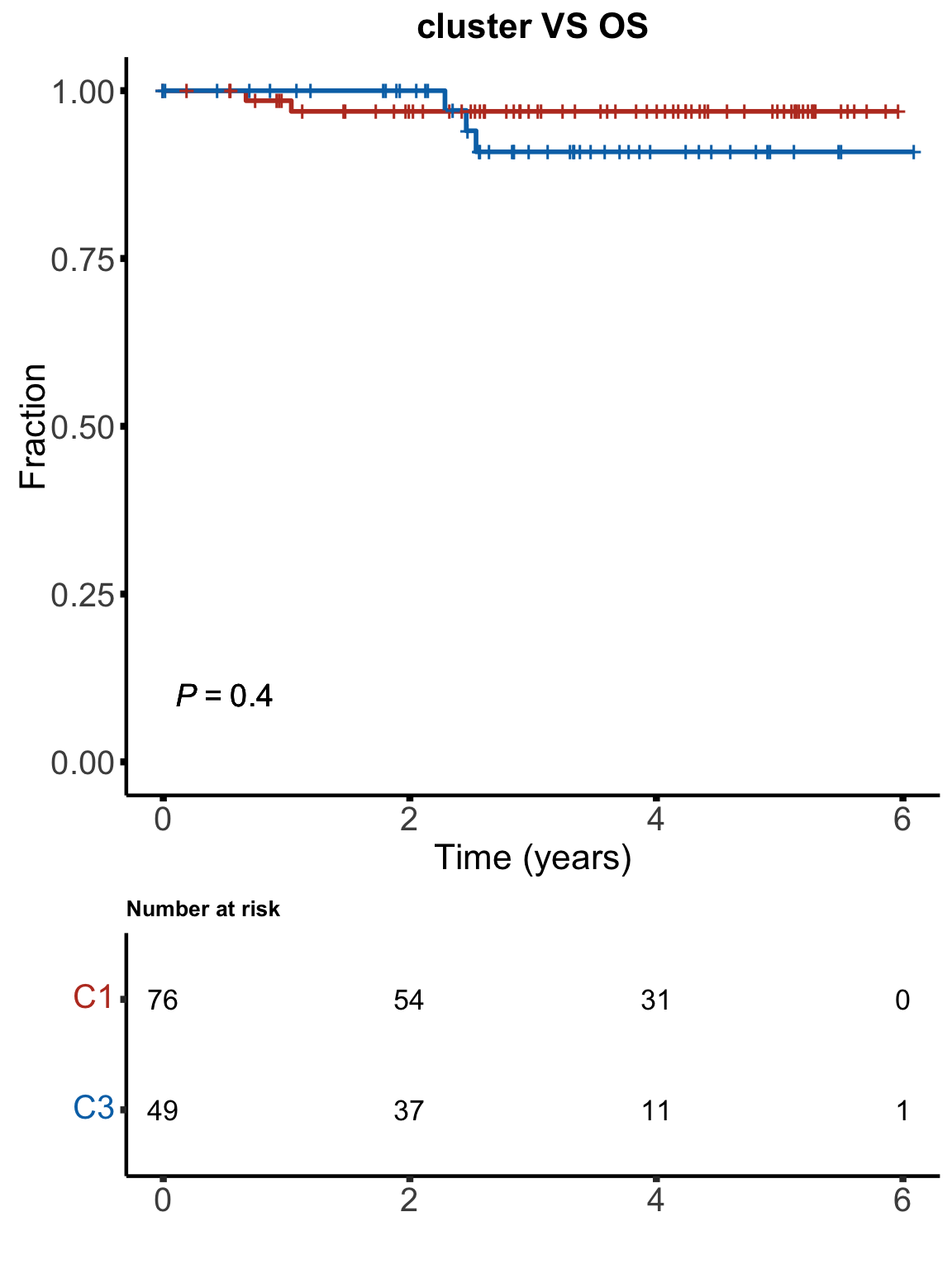 No significant associations between clinical outcomes and C1/C3 groups can be find. This suggests C1/C3 group can be either a subgroup only relates to drug response phenotype or C1/C3 relates to some confounding artefacts (e.g. samples processing, in vitro condition, spontaneous apoptosis …). This may need further investigation.
Association with treatment history
Only samples with BR therapy are enough for the test
load("../../var/inVivoEffect.RData")
testTab <- inVivoEffect %>% pivot_longer(-c(patientID, item)) %>%
  left_join(clusterTab, by = "patientID") %>%
  filter(cluster %in% c("C1","C3"), item == "BR", IGHV.status == "M")

table(testTab$name, testTab$cluster)
           C1 C3
  dropRate  5  7
  lymDrop   5  7
testRes <- group_by(testTab, name) %>% nest() %>%
mutate(m=map(data, ~t.test(value~cluster, ., var.equal = FALSE))) %>%
mutate(res = map(m, broom::tidy)) %>%
unnest(res)
testRes# A tibble: 2 × 13
# Groups: name [2]
name data m estimate estimate1 estimate2 statistic p.value
<chr> <list> <list> <dbl> <dbl> <dbl> <dbl> <dbl>
1 lymDrop <tibble> <htest> 0.561 1.89 1.33 2.20 0.0539
2 dropRate <tibble> <htest> 0.00420 0.0120 0.00781 1.78 0.140
# … with 5 more variables: parameter <dbl>, conf.low <dbl>, conf.high <dbl>,
# method <chr>, alternative <chr>ggplot(testTab, aes(x=cluster, y = value, col = cluster)) +
#geom_boxplot(outlier.shape = NA, width =0.3) +
geom_point(size=3) +
scale_color_manual(values = annoCol$cluster) +
facet_wrap(~name, scale = "free") +
theme_my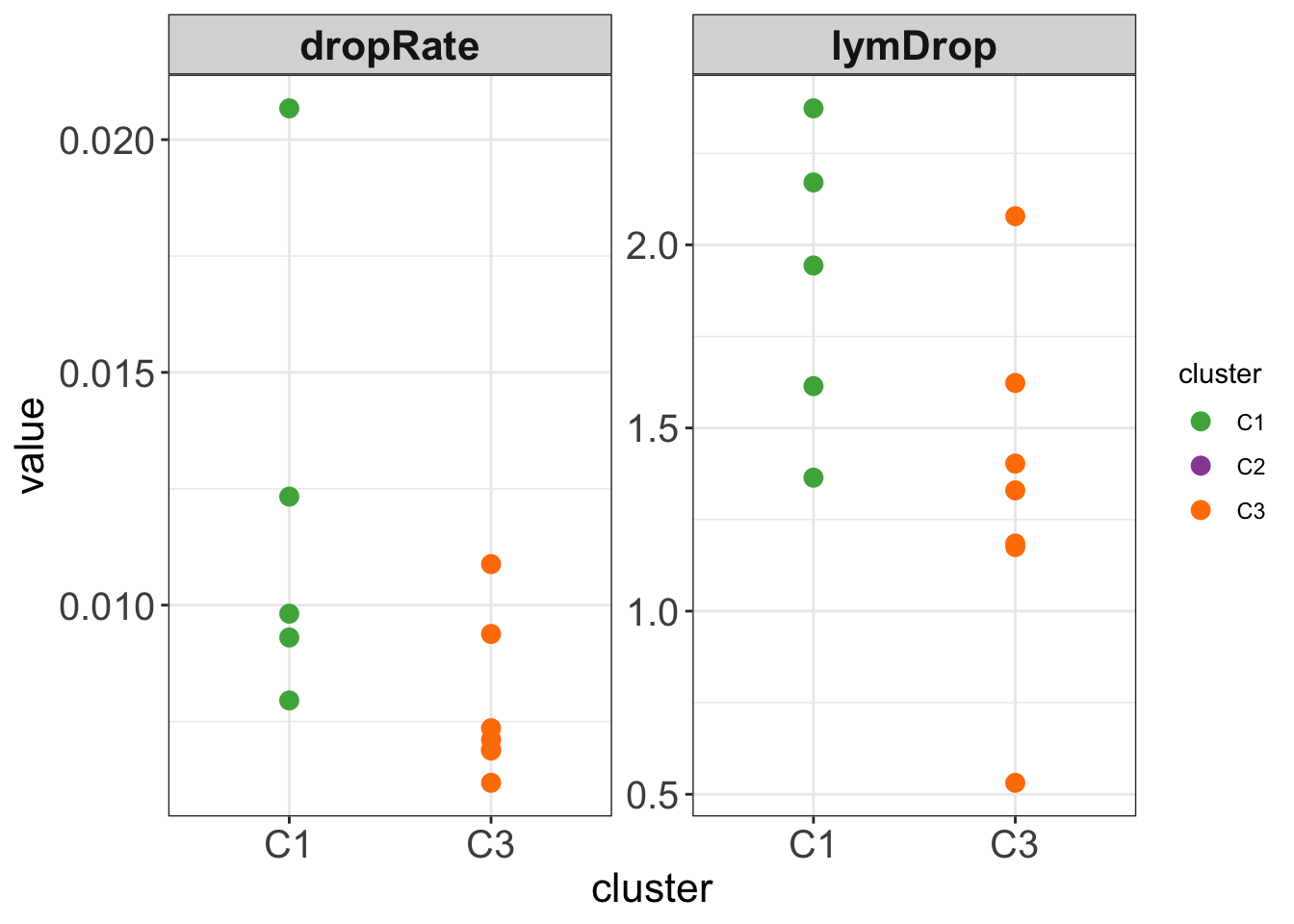 Perhaps too few samples, but the trend is interesting.
Compare the clustering results
load("../output/resConsClust.RData")
clustEMBL <- tibble(patientID = names(resConsClust[[3]]$consensusClass),
                    clusterEMBL = paste0("C",resConsClust[[3]]$consensusClass))

compareTab <- clusterTab %>% left_join(clustEMBL, by = "patientID")
table(compareTab$clusterEMBL, compareTab$cluster)
     C1 C2 C3
  C1 28  4 12
  C2  1 33  6
  C3  4  7  9
sessionInfo()R version 4.1.2 (2021-11-01)
Platform: x86_64-apple-darwin17.0 (64-bit)
Running under: macOS Big Sur 10.16
Matrix products: default
BLAS: /Library/Frameworks/R.framework/Versions/4.1/Resources/lib/libRblas.0.dylib
LAPACK: /Library/Frameworks/R.framework/Versions/4.1/Resources/lib/libRlapack.dylib
locale:
[1] en_US.UTF-8/en_US.UTF-8/en_US.UTF-8/C/en_US.UTF-8/en_US.UTF-8
attached base packages:
[1] stats4 stats graphics grDevices utils datasets methods
[8] base
other attached packages:
[1] forcats_0.5.1 stringr_1.4.0
[3] dplyr_1.0.7 purrr_0.3.4
[5] readr_2.1.1 tidyr_1.1.4
[7] tibble_3.1.6 tidyverse_1.3.1
[9] missForest_1.4 itertools_0.1-3
[11] iterators_1.0.13 foreach_1.5.1
[13] randomForest_4.6-14 Rtsne_0.15
[15] pheatmap_1.0.12 proDA_1.8.0
[17] DESeq2_1.34.0 SummarizedExperiment_1.24.0
[19] Biobase_2.54.0 MatrixGenerics_1.6.0
[21] matrixStats_0.61.0 GenomicRanges_1.46.1
[23] GenomeInfoDb_1.30.0 IRanges_2.28.0
[25] S4Vectors_0.32.3 BiocGenerics_0.40.0
[27] survminer_0.4.9 ggpubr_0.4.0
[29] ggplot2_3.3.5 survival_3.2-13
[31] cowplot_1.1.1 ConsensusClusterPlus_1.58.0
loaded via a namespace (and not attached):
[1] shinydashboard_0.7.2 utf8_1.2.2 tidyselect_1.1.1
[4] RSQLite_2.2.9 AnnotationDbi_1.56.2 htmlwidgets_1.5.4
[7] grid_4.1.2 BiocParallel_1.28.3 maxstat_0.7-25
[10] munsell_0.5.0 codetools_0.2-18 DT_0.20
[13] withr_2.4.3 colorspace_2.0-2 highr_0.9
[16] knitr_1.37 rstudioapi_0.13 ggsignif_0.6.3
[19] labeling_0.4.2 git2r_0.29.0 slam_0.1-50
[22] GenomeInfoDbData_1.2.7 KMsurv_0.1-5 bit64_4.0.5
[25] farver_2.1.0 rprojroot_2.0.2 vctrs_0.3.8
[28] generics_0.1.1 TH.data_1.1-0 xfun_0.29
[31] sets_1.0-20 markdown_1.1 R6_2.5.1
[34] ggbeeswarm_0.6.0 locfit_1.5-9.4 fgsea_1.20.0
[37] bitops_1.0-7 cachem_1.0.6 DelayedArray_0.20.0
[40] assertthat_0.2.1 promises_1.2.0.1 scales_1.1.1
[43] vroom_1.5.7 multcomp_1.4-18 beeswarm_0.4.0
[46] gtable_0.3.0 extraDistr_1.9.1 sandwich_3.0-1
[49] workflowr_1.7.0 rlang_0.4.12 genefilter_1.76.0
[52] splines_4.1.2 rstatix_0.7.0 broom_0.7.11
[55] BiocManager_1.30.16 yaml_2.2.1 abind_1.4-5
[58] modelr_0.1.8 crosstalk_1.2.0 backports_1.4.1
[61] httpuv_1.6.5 gridtext_0.1.4 relations_0.6-10
[64] tools_4.1.2 ellipsis_0.3.2 gplots_3.1.1
[67] jquerylib_0.1.4 RColorBrewer_1.1-2 Rcpp_1.0.8
[70] visNetwork_2.1.0 zlibbioc_1.40.0 RCurl_1.98-1.5
[73] zoo_1.8-9 haven_2.4.3 ggrepel_0.9.1
[76] cluster_2.1.2 exactRankTests_0.8-34 fs_1.5.2
[79] magrittr_2.0.1 data.table_1.14.2 reprex_2.0.1
[82] mvtnorm_1.1-3 shinyjs_2.1.0 hms_1.1.1
[85] mime_0.12 evaluate_0.14 xtable_1.8-4
[88] XML_3.99-0.8 readxl_1.3.1 gridExtra_2.3
[91] compiler_4.1.2 KernSmooth_2.23-20 crayon_1.4.2
[94] htmltools_0.5.2 mgcv_1.8-38 later_1.3.0
[97] tzdb_0.2.0 ggtext_0.1.1 geneplotter_1.72.0
[100] lubridate_1.8.0 DBI_1.1.2 dbplyr_2.1.1
[103] MASS_7.3-55 jyluMisc_0.1.5 BiocStyle_2.22.0
[106] Matrix_1.4-0 car_3.0-12 cli_3.1.1
[109] marray_1.72.0 igraph_1.2.11 parallel_4.1.2
[112] pkgconfig_2.0.3 km.ci_0.5-2 piano_2.10.0
[115] xml2_1.3.3 annotate_1.72.0 vipor_0.4.5
[118] bslib_0.3.1 XVector_0.34.0 drc_3.0-1
[121] rvest_1.0.2 digest_0.6.29 Biostrings_2.62.0
[124] fastmatch_1.1-3 rmarkdown_2.11 cellranger_1.1.0
[127] survMisc_0.5.5 shiny_1.7.1 gtools_3.9.2
[130] lifecycle_1.0.1 nlme_3.1-155 jsonlite_1.7.3
[133] carData_3.0-5 limma_3.50.0 fansi_1.0.2
[136] pillar_1.6.5 lattice_0.20-45 KEGGREST_1.34.0
[139] fastmap_1.1.0 httr_1.4.2 plotrix_3.8-2
[142] glue_1.6.1 png_0.1-7 bit_4.0.4
[145] stringi_1.7.6 sass_0.4.0 blob_1.2.2
[148] caTools_1.18.2 memoise_2.0.1