Consensus clustering analysis based on drug responses
Junyan Lu
6 April 2022
Last updated: 2022-04-06
Checks: 6 1
Knit directory: EMBL2016/analysis/
This reproducible R Markdown analysis was created with workflowr (version 1.7.0). The Checks tab describes the reproducibility checks that were applied when the results were created. The Past versions tab lists the development history.
The R Markdown is untracked by Git. To know which version of the R Markdown file created these results, you’ll want to first commit it to the Git repo. If you’re still working on the analysis, you can ignore this warning. When you’re finished, you can run wflow_publish to commit the R Markdown file and build the HTML.
Great job! The global environment was empty. Objects defined in the global environment can affect the analysis in your R Markdown file in unknown ways. For reproduciblity it’s best to always run the code in an empty environment.
The command set.seed(20210512) was run prior to running the code in the R Markdown file. Setting a seed ensures that any results that rely on randomness, e.g. subsampling or permutations, are reproducible.
Great job! Recording the operating system, R version, and package versions is critical for reproducibility.
Nice! There were no cached chunks for this analysis, so you can be confident that you successfully produced the results during this run.
Great job! Using relative paths to the files within your workflowr project makes it easier to run your code on other machines.
Great! You are using Git for version control. Tracking code development and connecting the code version to the results is critical for reproducibility.
The results in this page were generated with repository version 12d1722. See the Past versions tab to see a history of the changes made to the R Markdown and HTML files.
Note that you need to be careful to ensure that all relevant files for the analysis have been committed to Git prior to generating the results (you can use wflow_publish or wflow_git_commit). workflowr only checks the R Markdown file, but you know if there are other scripts or data files that it depends on. Below is the status of the Git repository when the results were generated:
Ignored files:
    Ignored:    .DS_Store
    Ignored:    .Rhistory
    Ignored:    analysis/.DS_Store
    Ignored:    analysis/.Rhistory
    Ignored:    analysis/boxplot_AUC.png
    Ignored:    analysis/consensus_clustering_noFit_cache/
    Ignored:    analysis/dose_curve.png
    Ignored:    analysis/targetDist.png
    Ignored:    analysis/toxivity_box.png
    Ignored:    analysis/volcano.png
    Ignored:    data/.DS_Store

Untracked files:
    Untracked:  analysis/AUC_CLL_IC50/
    Untracked:  analysis/BRAF_analysis.Rmd
    Untracked:  analysis/GSVA_analysis.Rmd
    Untracked:  analysis/NOTCH1_signature.Rmd
    Untracked:  analysis/autoluminescence.Rmd
    Untracked:  analysis/bar_plot_mixed.pdf
    Untracked:  analysis/bar_plot_mixed_noU1.pdf
    Untracked:  analysis/beatAML/
    Untracked:  analysis/cohortComposition_CLLsamples.pdf
    Untracked:  analysis/cohortComposition_allSamples.pdf
    Untracked:  analysis/consensus_clustering.Rmd
    Untracked:  analysis/consensus_clustering_CPS.Rmd
    Untracked:  analysis/consensus_clustering_IC50.Rmd
    Untracked:  analysis/consensus_clustering_beatAML.Rmd
    Untracked:  analysis/consensus_clustering_noFit.Rmd
    Untracked:  analysis/consensus_clusters.pdf
    Untracked:  analysis/disease_specific.Rmd
    Untracked:  analysis/dose_curve_selected.pdf
    Untracked:  analysis/genomic_association.Rmd
    Untracked:  analysis/genomic_association_allDisease.Rmd
    Untracked:  analysis/mean_autoluminescence_val.csv
    Untracked:  analysis/mean_autoluminescence_val.xlsx
    Untracked:  analysis/noFit_CLL/
    Untracked:  analysis/number_associations.pdf
    Untracked:  analysis/overview.Rmd
    Untracked:  analysis/plotCohort.Rmd
    Untracked:  analysis/preprocess.Rmd
    Untracked:  analysis/volcano_noBlocking.pdf
    Untracked:  code/utils.R
    Untracked:  data/BeatAML_Waves1_2/
    Untracked:  data/ic50Tab.RData
    Untracked:  data/newEMBL_20210806.RData
    Untracked:  data/patMeta.RData
    Untracked:  data/targetAnnotation_all.csv
    Untracked:  force_sync.sh
    Untracked:  output/resConsClust.RData
    Untracked:  output/resConsClust_aucFit.RData
    Untracked:  output/resConsClust_beatAML.RData
    Untracked:  output/resConsClust_cps.RData
    Untracked:  output/resConsClust_ic50.RData
    Untracked:  output/resConsClust_noFit.RData
    Untracked:  output/screenData.RData
    Untracked:  sync.sh

Unstaged changes:
    Modified:   _workflowr.yml
    Modified:   analysis/_site.yml
    Deleted:    analysis/about.Rmd
    Modified:   analysis/index.Rmd
    Deleted:    analysis/license.Rmd
Note that any generated files, e.g. HTML, png, CSS, etc., are not included in this status report because it is ok for generated content to have uncommitted changes.
There are no past versions. Publish this analysis with wflow_publish() to start tracking its development.
Load libraries and datasets
Perform consensus clustering to identify CLL subgroups with different drug response pattern
Pre-processing
Select CLL samples and use AUC as measures of drug effect
screenData <- ic50 %>% dplyr::rename(viab = normVal, viab.auc  = normVal_auc, conc = Concentration)
#Prepare data
viabMat <- screenData %>%
  filter(diagnosis %in% "CLL") %>% #only CLL
  group_by(patientID, Drug) %>% summarise(viab = mean(viab.auc, na.rm=TRUE)) %>%
  spread(key = patientID, value = "viab") %>% data.frame() %>%
  column_to_rownames("Drug") %>% as.matrix()
Estimate missing value percentage
missDrug <- rowSums(is.na(viabMat))
missPat <- colSums(is.na(viabMat))
Original dimension
dim(viabMat)[1] 66 184Keep drug that have non-NA values in at least 80% of samples
viabMatFilt <- viabMat[missDrug/ncol(viabMat) <= 0.2, ]Number of filtered dimensions
dim(viabMatFilt)[1] 64 184Run clustering with ConcsensusClustterPlus
# Impute missing values using missForest, as missing values are not allowed for consensus clustering
viabMatImp <- viabMatFilt
#Center each feature by median
d <- sweep(viabMatImp,1, apply(viabMatImp,1, median, na.rm=T))
#consensus clustering
resConsClust <- ConsensusClusterPlus(d, maxK=20, reps=100 , pItem=0.8, pFeature=1, title = "AUC_CLL_IC50",
clusterAlg="hc",distance="pearson",seed=2021, plot="png")
#plot clustering result
#icl = calcICL(resConsClust,title="AUC_CLL_CPS1000",plot="png")
#save results for later use
save(viabMatImp, resConsClust, file = "../output/resConsClust_ic50.RData")Based on delta curve, three clusters would be most appropriate
load("../output/resConsClust_ic50.RData")Post-processing consensus clustering results
Select samples with clustering consensus over 80%
k=3
conMat <- resConsClust[[k]]$consensusMatrix
conClust <- resConsClust[[k]]$consensusClass
colnames(conMat) <- colnames(viabMatImp)

#change cluster number to be consistent with EMBL screen reuslts
conClust <- case_when(conClust == 1 ~ 2,
                      conClust == 2 ~ 3,
                      conClust == 3 ~ 1)
names(conClust) <- colnames(conMat)
Visualization
clusterTab <- tibble(patientID = colnames(conMat),
cluster = paste0("C",conClust),
IGHV.status = patMeta[match(names(conClust),patMeta$Patient.ID),]$IGHV.status,
Mclust = patMeta[match(names(conClust),patMeta$Patient.ID),]$Methylation_Cluster,
trisomy12 = patMeta[match(names(conClust),patMeta$Patient.ID),]$trisomy12)
colAnno <- clusterTab %>% data.frame() %>% column_to_rownames("patientID")
pheatmap(conMat, annotation_col = colAnno, method = "average", clustering_distance_rows = "correlation", clustering_distance_cols = "correlation")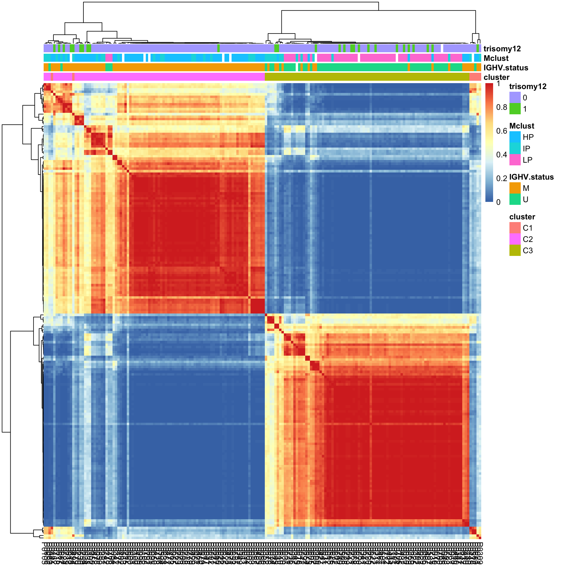 Based on the heatmap, C2 is primarily U-CLL samples while C1 and C2 are primarily M-CLL samples
Visualization (for abstract)
colAnnoAlt <- data.frame(row.names = colnames(conMat),
                      cluster = paste0("C",conClust),
                      IGHV.status = patMeta[match(names(conClust),patMeta$Patient.ID),]$IGHV.status)

annoCol <- list(IGHV.status = c(M = "#E41A1C", U = "#377EB8"),
                cluster = c(C1 = "#4DAF4A", C2 = "#984EA3", C3 = "#FF7F00"))
#pdf("consensus_clusters.pdf", height = 4, width = 5)
pheatmap(conMat, annotation_col = colAnnoAlt, method = "average", clustering_distance_rows = "correlation", clustering_distance_cols = "correlation",
         color = blues9, treeheight_row = 0, treeheight_col = 1, border_color = NA, show_colnames = FALSE, annotation_colors = annoCol)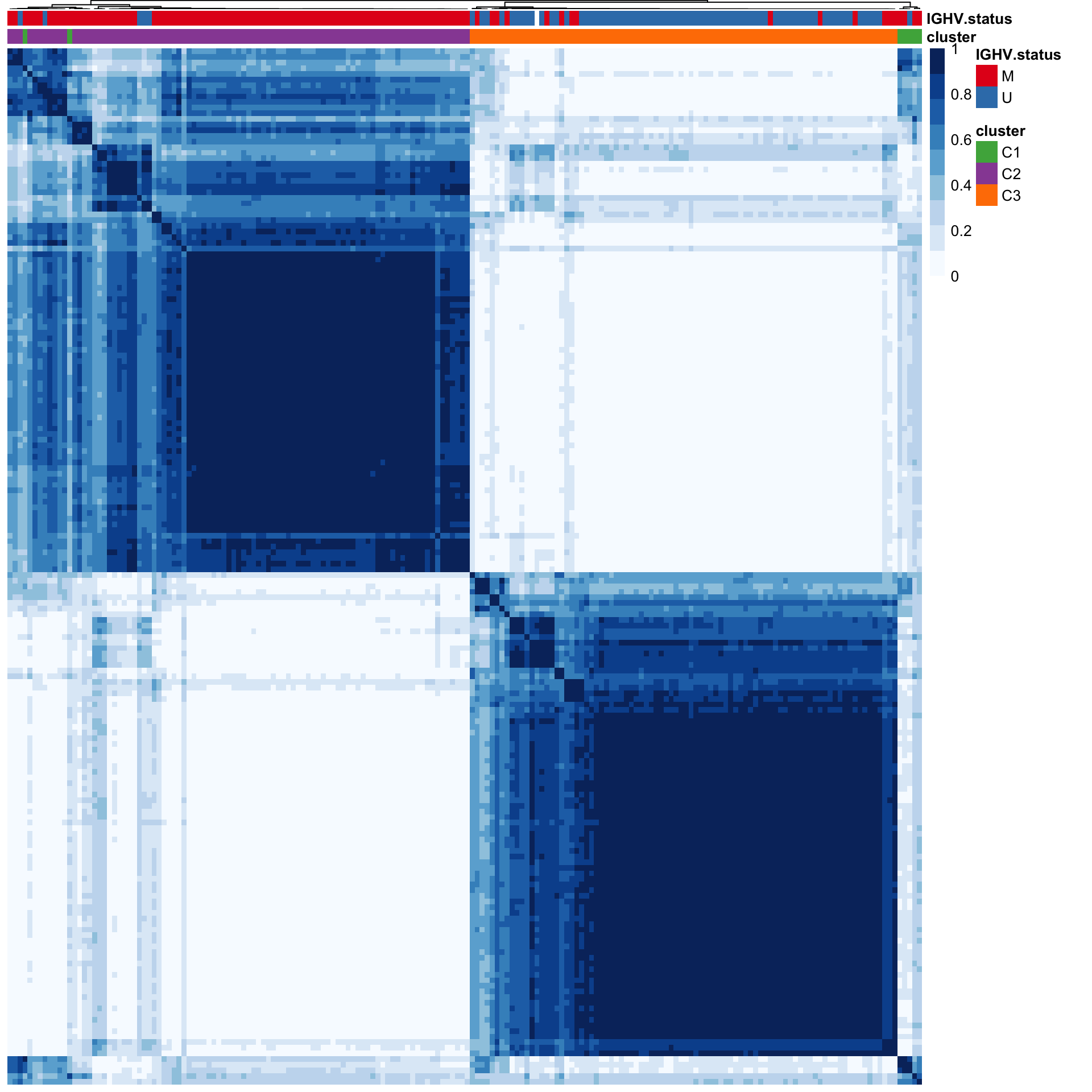
#dev.off()C1 and C2 groups are predominately M-CLL samples
table(clusterTab$cluster, clusterTab$IGHV.status)
      M  U
  C1  6  1
  C2 86  5
  C3 14 71
plotTab <- clusterTab %>%
filter(!is.na(IGHV.status)) %>%
group_by(cluster, IGHV.status) %>%
summarise(n=length(patientID))
ggplot(plotTab, aes(x=cluster,y=n, fill = IGHV.status)) +
geom_bar(stat="identity", postion = "stack") +
xlab("number of samples") +
scale_fill_manual(values = c(M = "#E41A1C", U = "#377EB8")) +
theme_my +
theme(legend.position = "bottom")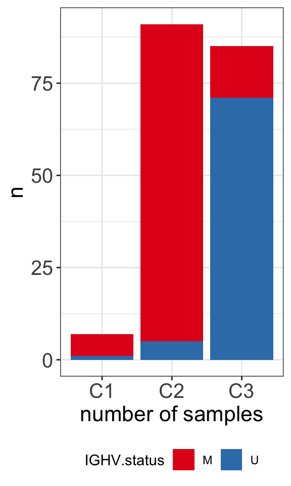
C1 and C2 groups are predominately M-CLL samples
table(clusterTab$cluster, clusterTab$Mclust)
     HP IP LP
  C1  3  3  0
  C2 62 20  3
  C3  7 12 64
plotTab <- clusterTab %>%
filter(!is.na(Mclust)) %>%
group_by(cluster, Mclust) %>%
summarise(n=length(patientID))
ggplot(plotTab, aes(x=cluster,y=n, fill = Mclust)) +
geom_bar(stat="identity", postion = "stack") +
xlab("number of samples") +
#scale_fill_manual(values = c(M = "#E41A1C", U = "#377EB8")) +
theme_my +
theme(legend.position = "bottom")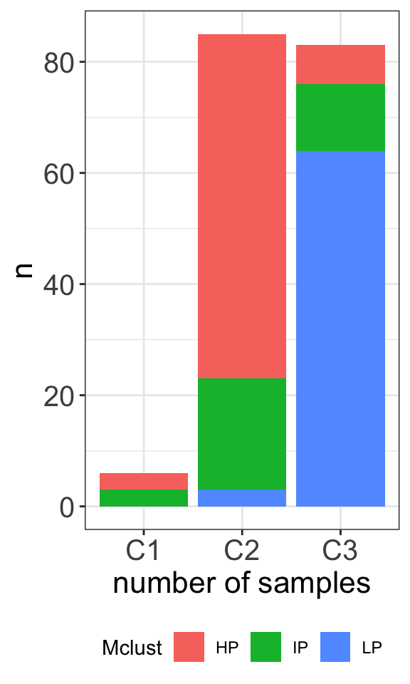
Both C1 and C2 are M-CLL samples. How they are different in terms of drug responses and why they are different?
For the ease of comparison with other datasets, the name of C2 and C3 will be interchanged.
clusterTab <- mutate(clusterTab,
                     cluster = case_when(
                       cluster == "C2" ~ "C3",
                       cluster == "C3" ~ "C2",
                       cluster == "C1" ~ "C1"
                     ))
T-SNE visualization
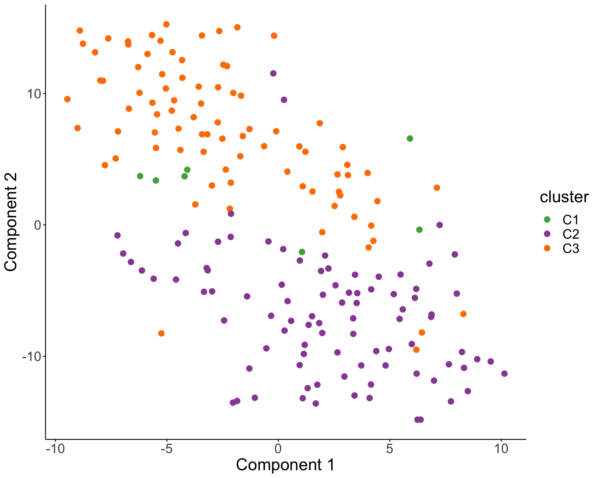
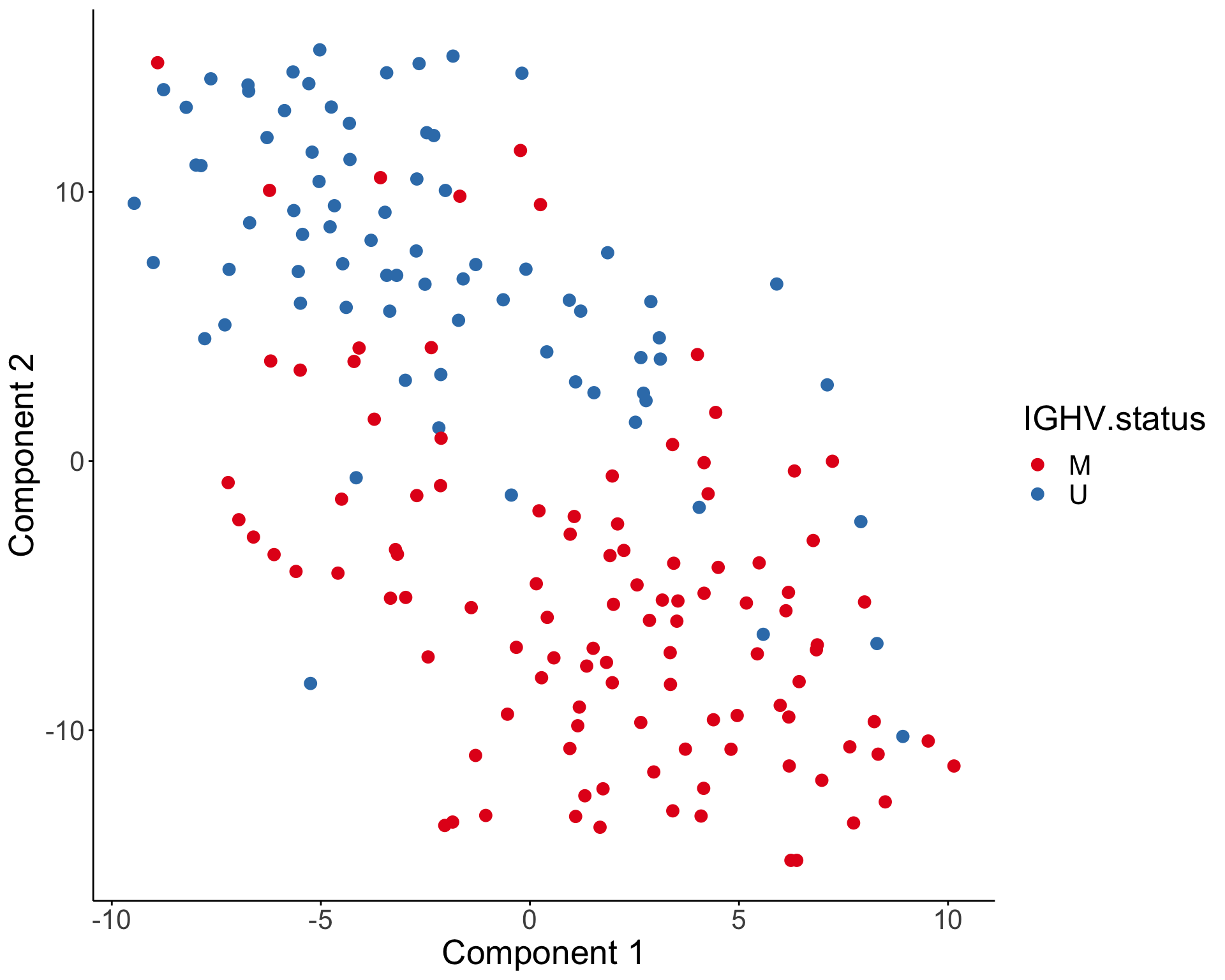
Characterize the drug response phenotypes of C1 and C3 subgroup within M-CLL samples
Identify drugs that show differential responses between C1 and C3 in M-CLL samples
clusterTab <- clusterTab %>%
  mutate(sampleID = screenData[match(patientID, screenData$patientID),]$sampleID)

testTabAll <- screenData %>%
  filter(diagnosis %in% "CLL") %>% #only CLL
  group_by(patientID, Drug) %>% summarise(viab = mean(viab.auc, na.rm=TRUE)) %>%
  left_join(clusterTab, by = "patientID")

testTab <- testTabAll %>%
  filter(cluster %in% c("C1","C3"),
         IGHV.status %in% "M",
         !is.na(viab)) %>%
  mutate(cluster =factor(cluster, levels = c("C1","C3")))

#at least five samples if each cluster for each drug, this is because for some drugs the AUC could not be fitted
drugFilt <- group_by(testTab, cluster, Drug) %>%
  summarise(n = length(!is.na(viab))) %>%
  pivot_wider(names_from = cluster, values_from = n) %>%
  filter(C1>=5 & C3>=5)

testTab <- filter(testTab, Drug %in% drugFilt$Drug)
resTab <- testTab %>% group_by(Drug) %>% nest() %>%
mutate(m=map(data, ~t.test(viab~cluster, ., var.equal=TRUE))) %>%
mutate(res = map(m, broom::tidy)) %>%
unnest(res) %>% ungroup() %>%
select(Drug, estimate, p.value, estimate1, estimate2) %>%
mutate(p.adj = p.adjust(p.value, method = "BH"), log2FC = log2(estimate2/estimate1)) %>%
arrange(p.value)Volcano plot
plotTabVol <- resTab %>%
  mutate(direction = case_when(p.adj > 0.01 ~ "n.s.",
                               p.adj < 0.01 & log2FC <0 ~ "sensitive in C3",
                               p.adj < 0.01 & log2FC >0 ~ "resistent in C3"))

#label top 12 drugs judged by pvalue
topDrug <- arrange(resTab, p.value)$Drug[1:12]
plotTabVol <- mutate(plotTabVol, drugLabel = ifelse(Drug %in% topDrug, as.character(Drug), ""))

ggplot(plotTabVol, aes(y=-log10(p.adj), x= log2FC)) +
  geom_point(aes(col = direction)) +
  geom_hline(yintercept = 2, linetype ="dashed") +
  ggrepel::geom_text_repel(aes(label = drugLabel),max.overlaps=100) +
  scale_color_manual(values = c(n.s. = "grey50", `sensitive in C3` = "blue", `resistent in C3` = "red")) +
  xlim(-0.8,0.8) +
  ggtitle("Drug sensitivity between C1 and C3\n(within M-CLL samples)") +
  theme_my +
  theme(plot.title = element_text(hjust=0.5, size=15, face ="bold"))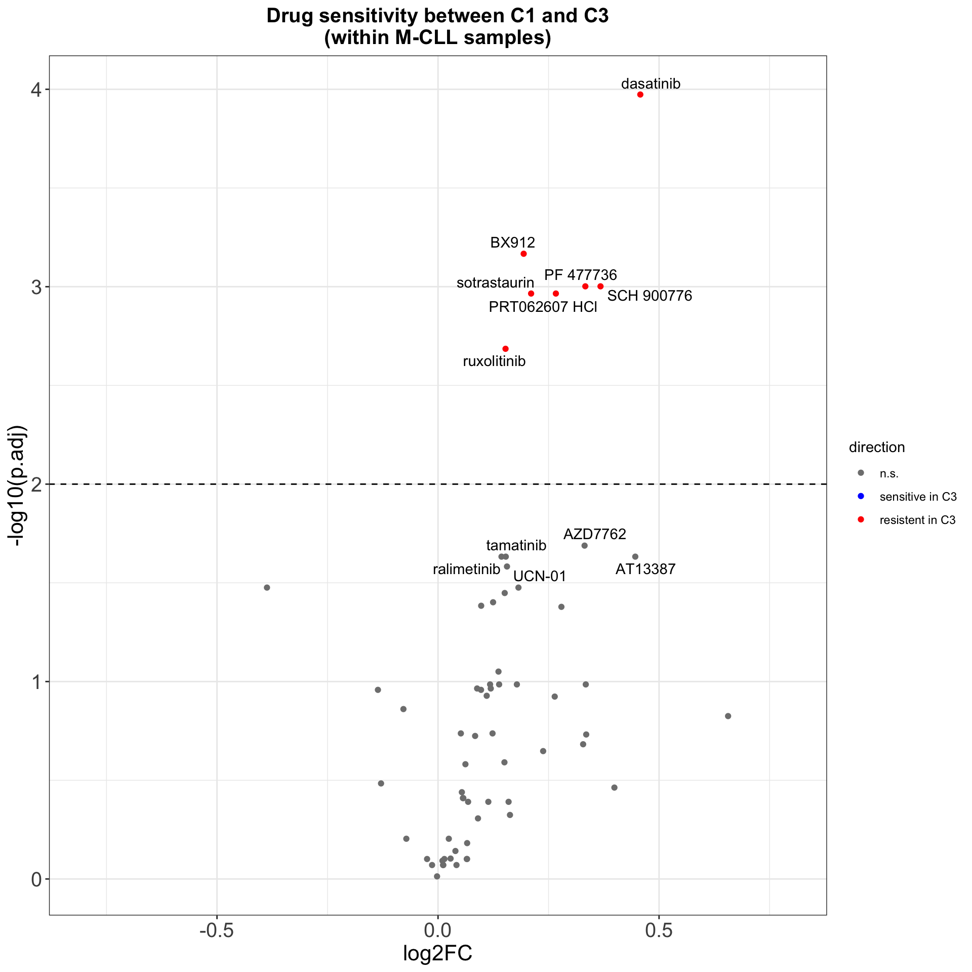
ggsave("volcano.png", height = 5, width = 6)Drug with 1% FDR and abs(log2FC) > 0.5 are labeled
A list of all drugs associated with C1/C3 subgroups
10% FDR cut-off is used
resTab %>% filter(p.adj < 0.1) %>%
  mutate_if(is.numeric, formatC, digits=2) %>%
  DT::datatable()
Boxplots
Only M-CLL samples that belong to C1 and C3 group
drugList <- filter(plotTabVol, drugLabel != "")$Drug
plotTabBox <- filter(testTab, Drug %in% drugList)
ggplot(plotTabBox, aes(x=cluster, y = viab)) +
  geom_boxplot(outlier.shape = NA, aes(fill = cluster)) + ggbeeswarm::geom_quasirandom() +
  facet_wrap(~Drug) +
  theme_my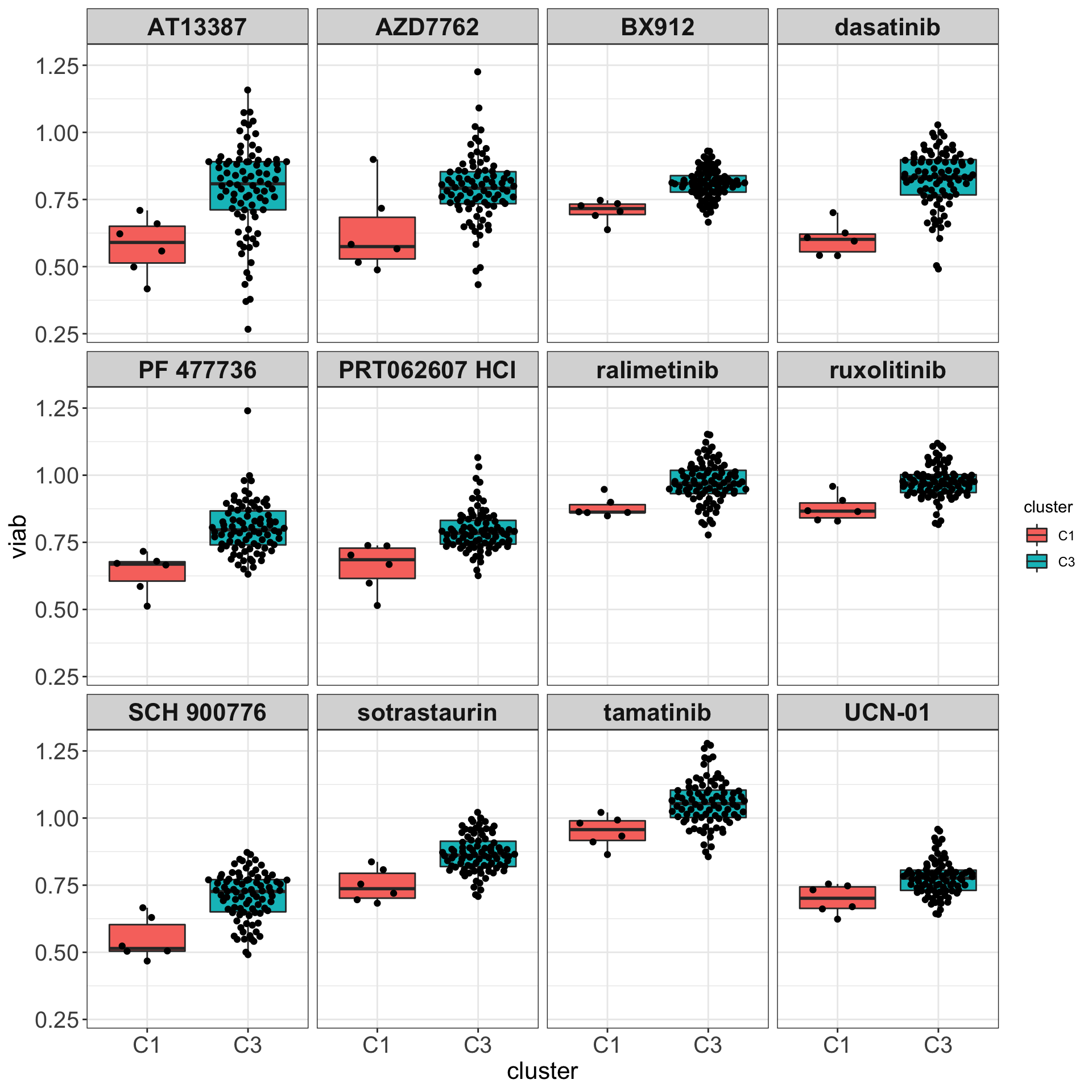
All samples and colored by their IGHV status
drugList <- filter(plotTabVol, drugLabel != "")$Drug
plotTabBox <- filter(testTabAll, Drug %in% drugList, !is.na(IGHV.status))
ggplot(plotTabBox, aes(x=cluster, y = viab)) +
  geom_boxplot(outlier.shape = NA) +
  ggbeeswarm::geom_quasirandom(aes(col= IGHV.status)) +
  scale_color_manual(values = c(M = "#E41A1C", U = "#377EB8")) +
  facet_wrap(~Drug, ncol=4) +
  ylab("Viability (AUC)") + xlab("Clusters") +
  theme_my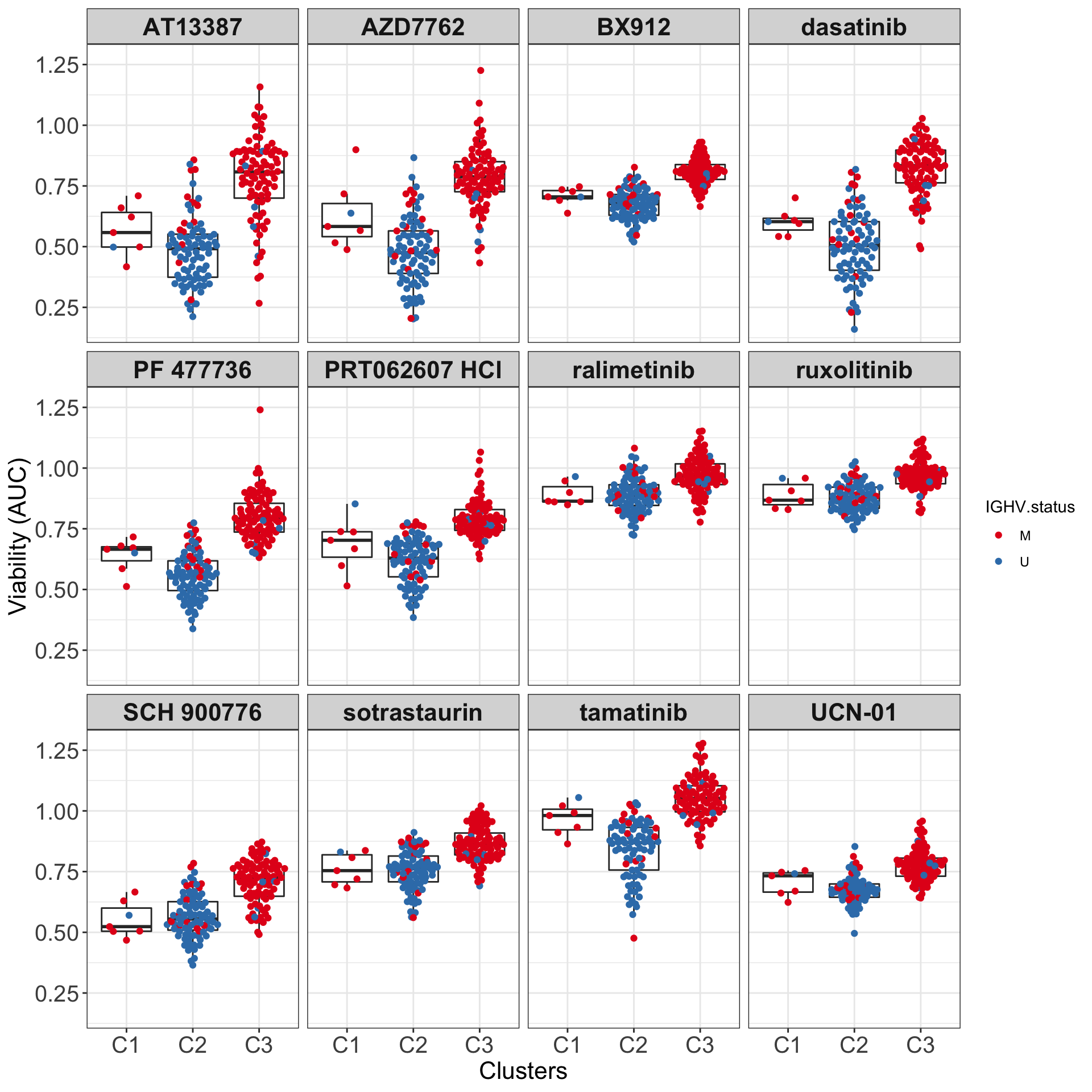
ggsave("boxplot_AUC.png", height = 6, width = 12)Boxplots (C1, C2 and C3) colored by methylation cluster
drugList <- filter(plotTabVol, drugLabel != "")$Drug
plotTabBox <- filter(testTabAll, Drug %in% drugList)
ggplot(plotTabBox, aes(x=cluster, y = viab)) +
geom_boxplot(outlier.shape = NA) +
ggbeeswarm::geom_quasirandom(aes(col= Mclust)) +
facet_wrap(~Drug) +
theme_my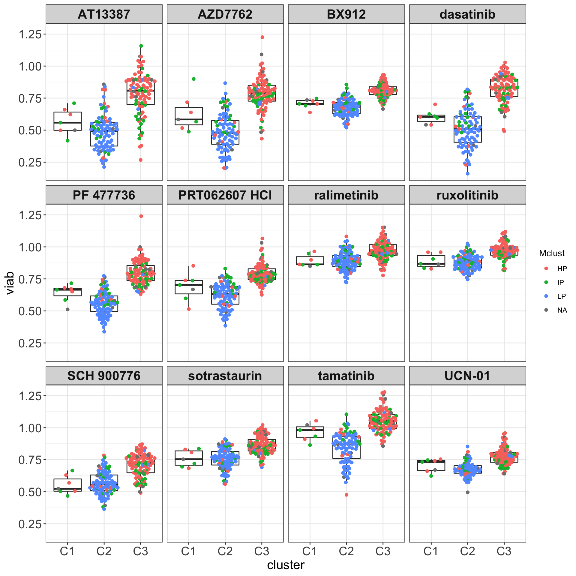 The methylation groups do not explain the difference between C1 and C3 groups.
Dose-response curves
drugList <- filter(plotTabVol, drugLabel != "")$Drug
plotTabCurve <- filter(screenData, Drug %in% drugList) %>%
  left_join(clusterTab) %>% filter(cluster %in% c("C1","C3"))
ggplot(plotTabCurve, aes(x=conc, y = viab, col = cluster, group = sampleID)) +
  #geom_smooth(geom="line", method = "loess", se=FALSE, alpha=0.5, size=0.5) +
  scale_x_log10() +
  geom_line() +
  scale_color_manual(values = c(C1 = "#4DAF4A", C2 = "#984EA3", C3 = "#FF7F00")) +
  facet_wrap(~Drug, ncol=4) +
  theme_my + xlab("concentration") + ylab("viability")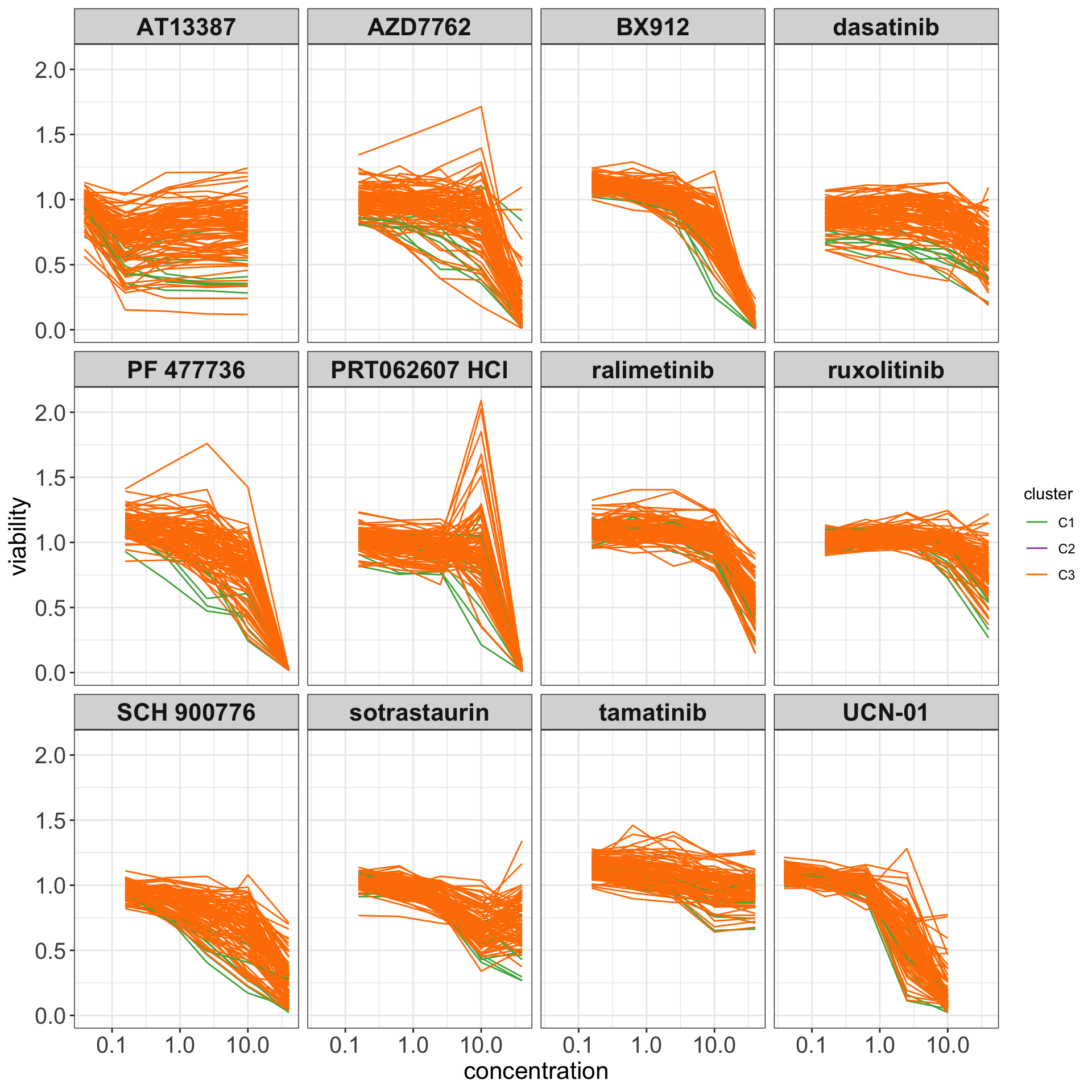
ggsave("dose_curve.png", height = 6, width = 12)General toxicity and group
resTabSig <- filter(resTab, p.adj < 0.1 )
meanViabTab <- filter(screenData,  Drug %in% resTab$Drug) %>%
  group_by(Drug) %>% summarise(meanViab = mean(viab.auc, na.rm=TRUE)) %>%
  mutate(ifSig = ifelse(Drug %in% resTabSig$Drug,"yes","no"))

t.test(meanViab ~ ifSig, meanViabTab)
    Welch Two Sample t-test

data:  meanViab by ifSig
t = -0.90572, df = 54.701, p-value = 0.3691
alternative hypothesis: true difference in means between group no and group yes is not equal to 0
95 percent confidence interval:
 -0.12952803  0.04889874
sample estimates:
 mean in group no mean in group yes
        0.7258699         0.7661845
ggplot(meanViabTab, aes(x=ifSig, y=meanViab)) +
geom_boxplot() + geom_point() +
theme_my +
ylab("mean viability among all samples") + xlab("Associated with C1/C3 clusters")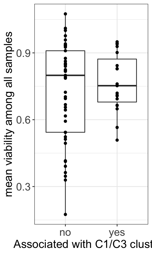
#ggsave("toxivity_box.png", width = 5, height = 4)
sessionInfo()R version 4.1.2 (2021-11-01)
Platform: x86_64-apple-darwin17.0 (64-bit)
Running under: macOS Big Sur 10.16
Matrix products: default
BLAS: /Library/Frameworks/R.framework/Versions/4.1/Resources/lib/libRblas.0.dylib
LAPACK: /Library/Frameworks/R.framework/Versions/4.1/Resources/lib/libRlapack.dylib
locale:
[1] en_US.UTF-8/en_US.UTF-8/en_US.UTF-8/C/en_US.UTF-8/en_US.UTF-8
attached base packages:
[1] stats4 stats graphics grDevices utils datasets methods
[8] base
other attached packages:
[1] forcats_0.5.1 stringr_1.4.0
[3] dplyr_1.0.7 purrr_0.3.4
[5] readr_2.1.1 tidyr_1.1.4
[7] tibble_3.1.6 tidyverse_1.3.1
[9] missForest_1.4 itertools_0.1-3
[11] iterators_1.0.13 foreach_1.5.1
[13] randomForest_4.6-14 Rtsne_0.15
[15] pheatmap_1.0.12 proDA_1.8.0
[17] DESeq2_1.34.0 SummarizedExperiment_1.24.0
[19] Biobase_2.54.0 MatrixGenerics_1.6.0
[21] matrixStats_0.61.0 GenomicRanges_1.46.1
[23] GenomeInfoDb_1.30.0 IRanges_2.28.0
[25] S4Vectors_0.32.3 BiocGenerics_0.40.0
[27] survminer_0.4.9 ggpubr_0.4.0
[29] ggplot2_3.3.5 survival_3.2-13
[31] cowplot_1.1.1 ConsensusClusterPlus_1.58.0
loaded via a namespace (and not attached):
[1] readxl_1.3.1 backports_1.4.1 workflowr_1.7.0
[4] splines_4.1.2 crosstalk_1.2.0 BiocParallel_1.28.3
[7] digest_0.6.29 htmltools_0.5.2 fansi_1.0.2
[10] magrittr_2.0.1 memoise_2.0.1 cluster_2.1.2
[13] tzdb_0.2.0 Biostrings_2.62.0 annotate_1.72.0
[16] modelr_0.1.8 colorspace_2.0-2 ggrepel_0.9.1
[19] blob_1.2.2 rvest_1.0.2 haven_2.4.3
[22] xfun_0.29 crayon_1.4.2 RCurl_1.98-1.5
[25] jsonlite_1.7.3 genefilter_1.76.0 zoo_1.8-9
[28] glue_1.6.1 gtable_0.3.0 zlibbioc_1.40.0
[31] XVector_0.34.0 DelayedArray_0.20.0 car_3.0-12
[34] abind_1.4-5 scales_1.1.1 DBI_1.1.2
[37] rstatix_0.7.0 Rcpp_1.0.8 xtable_1.8-4
[40] bit_4.0.4 km.ci_0.5-2 DT_0.20
[43] htmlwidgets_1.5.4 httr_1.4.2 RColorBrewer_1.1-2
[46] ellipsis_0.3.2 pkgconfig_2.0.3 XML_3.99-0.8
[49] farver_2.1.0 sass_0.4.0 dbplyr_2.1.1
[52] locfit_1.5-9.4 utf8_1.2.2 tidyselect_1.1.1
[55] labeling_0.4.2 rlang_0.4.12 later_1.3.0
[58] AnnotationDbi_1.56.2 munsell_0.5.0 cellranger_1.1.0
[61] tools_4.1.2 cachem_1.0.6 cli_3.1.1
[64] generics_0.1.1 RSQLite_2.2.9 broom_0.7.11
[67] evaluate_0.14 fastmap_1.1.0 yaml_2.2.1
[70] knitr_1.37 bit64_4.0.5 fs_1.5.2
[73] survMisc_0.5.5 KEGGREST_1.34.0 xml2_1.3.3
[76] BiocStyle_2.22.0 compiler_4.1.2 rstudioapi_0.13
[79] beeswarm_0.4.0 png_0.1-7 ggsignif_0.6.3
[82] reprex_2.0.1 geneplotter_1.72.0 bslib_0.3.1
[85] stringi_1.7.6 highr_0.9 lattice_0.20-45
[88] Matrix_1.4-0 KMsurv_0.1-5 vctrs_0.3.8
[91] pillar_1.6.5 lifecycle_1.0.1 BiocManager_1.30.16
[94] jquerylib_0.1.4 data.table_1.14.2 bitops_1.0-7
[97] httpuv_1.6.5 R6_2.5.1 promises_1.2.0.1
[100] gridExtra_2.3 vipor_0.4.5 codetools_0.2-18
[103] assertthat_0.2.1 rprojroot_2.0.2 withr_2.4.3
[106] GenomeInfoDbData_1.2.7 parallel_4.1.2 hms_1.1.1
[109] grid_4.1.2 rmarkdown_2.11 carData_3.0-5
[112] git2r_0.29.0 lubridate_1.8.0 ggbeeswarm_0.6.0