Consensus clustering analysis based on drug responses
Junyan Lu
31 March 2023
Last updated: 2023-03-31
Checks: 5 2
Knit directory: EMBL2016/analysis/
This reproducible R Markdown analysis was created with workflowr (version 1.7.0). The Checks tab describes the reproducibility checks that were applied when the results were created. The Past versions tab lists the development history.
The R Markdown is untracked by Git. To know which version of the R
Markdown file created these results, you’ll want to first commit it to
the Git repo. If you’re still working on the analysis, you can ignore
this warning. When you’re finished, you can run
wflow_publish to commit the R Markdown file and build the
HTML.
Great job! The global environment was empty. Objects defined in the global environment can affect the analysis in your R Markdown file in unknown ways. For reproduciblity it’s best to always run the code in an empty environment.
The command set.seed(20210512) was run prior to running
the code in the R Markdown file. Setting a seed ensures that any results
that rely on randomness, e.g. subsampling or permutations, are
reproducible.
Great job! Recording the operating system, R version, and package versions is critical for reproducibility.
- unnamed-chunk-57
- unnamed-chunk-59
- unnamed-chunk-60
- unnamed-chunk-66
- unnamed-chunk-77
To ensure reproducibility of the results, delete the cache directory
consensus_clustering_noFit_cache and re-run the analysis.
To have workflowr automatically delete the cache directory prior to
building the file, set delete_cache = TRUE when running
wflow_build() or wflow_publish().
Great job! Using relative paths to the files within your workflowr project makes it easier to run your code on other machines.
Great! You are using Git for version control. Tracking code development and connecting the code version to the results is critical for reproducibility.
The results in this page were generated with repository version 12d1722. See the Past versions tab to see a history of the changes made to the R Markdown and HTML files.
Note that you need to be careful to ensure that all relevant files for
the analysis have been committed to Git prior to generating the results
(you can use wflow_publish or
wflow_git_commit). workflowr only checks the R Markdown
file, but you know if there are other scripts or data files that it
depends on. Below is the status of the Git repository when the results
were generated:
Ignored files:
    Ignored:    .DS_Store
    Ignored:    .Rhistory
    Ignored:    .Rproj.user/
    Ignored:    analysis/.DS_Store
    Ignored:    analysis/.RData
    Ignored:    analysis/.Rhistory
    Ignored:    analysis/CDK_analysis_cache/
    Ignored:    analysis/boxplot_AUC.png
    Ignored:    analysis/consensus_clustering_CPS_cache/
    Ignored:    analysis/consensus_clustering_noFit_cache/
    Ignored:    analysis/dose_curve.png
    Ignored:    analysis/targetDist.png
    Ignored:    analysis/toxivity_box.png
    Ignored:    analysis/volcano.png
    Ignored:    data/.DS_Store
    Ignored:    output/.DS_Store

Untracked files:
    Untracked:  analysis/AUC_CLL_IC50/
    Untracked:  analysis/BRAF_analysis.Rmd
    Untracked:  analysis/CDK_analysis.Rmd
    Untracked:  analysis/GSVA_analysis.Rmd
    Untracked:  analysis/MOFA_analysis.Rmd
    Untracked:  analysis/NOTCH1_signature.Rmd
    Untracked:  analysis/autoluminescence.Rmd
    Untracked:  analysis/bar_plot_mixed_noU1.pdf
    Untracked:  analysis/beatAML/
    Untracked:  analysis/consensus_clustering.Rmd
    Untracked:  analysis/consensus_clustering_CPS.Rmd
    Untracked:  analysis/consensus_clustering_IC50.Rmd
    Untracked:  analysis/consensus_clustering_beatAML.Rmd
    Untracked:  analysis/consensus_clustering_noFit.Rmd
    Untracked:  analysis/coxResTab.RData
    Untracked:  analysis/disease_specific.Rmd
    Untracked:  analysis/drugScreens_reproducibility.Rmd
    Untracked:  analysis/genomic_association.Rmd
    Untracked:  analysis/genomic_association_IC50.Rmd
    Untracked:  analysis/genomic_association_allDisease.Rmd
    Untracked:  analysis/noFit_CLL/
    Untracked:  analysis/outcome_associations.Rmd
    Untracked:  analysis/overview.Rmd
    Untracked:  analysis/plotCohort.Rmd
    Untracked:  analysis/preprocess.Rmd
    Untracked:  analysis/volcano_drugGene.pdf
    Untracked:  code/utils.R
    Untracked:  data/BeatAML_Waves1_2/
    Untracked:  data/ic50Tab.RData
    Untracked:  data/newEMBL_20210806.RData
    Untracked:  data/patMeta.RData
    Untracked:  data/targetAnnotation_all.csv
    Untracked:  output/consClust_CPS.csv
    Untracked:  output/consClust_EMBL2016.csv
    Untracked:  output/consClust_IC50.csv
    Untracked:  output/gene_associations/
    Untracked:  output/mofaRes.rds
    Untracked:  output/resConsClust.RData
    Untracked:  output/resConsClust_aucFit.RData
    Untracked:  output/resConsClust_beatAML.RData
    Untracked:  output/resConsClust_cps.RData
    Untracked:  output/resConsClust_ic50.RData
    Untracked:  output/resConsClust_noFit.RData
    Untracked:  output/screenData.RData

Unstaged changes:
    Modified:   _workflowr.yml
    Modified:   analysis/_site.yml
    Deleted:    analysis/about.Rmd
    Modified:   analysis/index.Rmd
    Deleted:    analysis/license.Rmd
Note that any generated files, e.g. HTML, png, CSS, etc., are not included in this status report because it is ok for generated content to have uncommitted changes.
There are no past versions. Publish this analysis with
wflow_publish() to start tracking its development.
Load libraries and datasets
Perform consensus clustering to identify CLL subgroups with different drug response pattern
Pre-processing
Remove drugs with self-lumination
screenData <- filter(screenData, !problemDrug)Select CLL samples and use AUC under lines
#Prepare data
viabMat <- screenData %>%
  filter(diagnosis %in% "CLL") %>% #only CLL
  distinct(patientID, Drug, .keep_all = TRUE) %>%
  select(patientID, Drug, viab.auc) %>%
  #group_by(patientID, Drug) %>% summarise(viab = mean(viab.auc, na.rm=TRUE)) %>%
  spread(key = patientID, value = "viab.auc") %>% data.frame() %>%
  column_to_rownames("Drug") %>% as.matrix()
Estimate missing value percentage
missDrug <- rowSums(is.na(viabMat))
missPat <- colSums(is.na(viabMat))
Original dimension
dim(viabMat)[1] 391 132Keep drug that have non-NA values in at least 80% of samples (in this version, no drugs will be removed at this step)
viabMatFilt <- viabMat[missDrug/ncol(viabMat) <= 0.2, ]Remove drugs do not show variations (not used)
#sds <- genefilter::rowSds(viabMatFilt, na.rm=TRUE)
#viabMatFilt <- viabMatFilt[sds > genefilter::shorth(sds),]
Number of filtered dimensions
dim(viabMatFilt)[1] 391 132Run clustering with ConcsensusClustterPlus
# Impute missing values using missForest, as missing values are not allowed for consensus clustering
set.seed(2021)
impForest <- missForest(t(viabMatFilt))
viabMatImp <- t(impForest$ximp)
#Center each feature by median
d <- sweep(viabMatImp,1, apply(viabMatImp,1, median, na.rm=T))
#consensus clustering
resConsClust <- ConsensusClusterPlus(d, maxK=20, reps=1000 , pItem=0.8, pFeature=1, title = "noFit_CLL",
clusterAlg="hc",distance="pearson",seed=2021, plot="png")
#plot clustering result
icl = calcICL(resConsClust,title="noFit_CLL",plot="png")
#save results for later use
save(viabMatImp, resConsClust, file = "../output/resConsClust_noFit.RData")Based on delta curve, three clusters would be most appropriate
Load saved data
load("../output/resConsClust_noFit.RData")Post-processing consensus clustering results
Select samples with clustering consensus over 80%
k=3
conMat <- resConsClust[[k]]$consensusMatrix
conClust <- resConsClust[[k]]$consensusClass
colnames(conMat) <- colnames(viabMatImp)
Visualization
clusterTab <- tibble(patientID = colnames(conMat),
                      cluster = paste0("C",conClust),
                      IGHV.status = patMeta[match(names(conClust),patMeta$Patient.ID),]$IGHV.status,
                      Mclust = patMeta[match(names(conClust),patMeta$Patient.ID),]$Methylation_Cluster,
                      trisomy12 = patMeta[match(names(conClust),patMeta$Patient.ID),]$trisomy12,
                     sampleID = screenData[match(patientID, screenData$patientID),]$sampleID
                     )


#add sample year information
yearTab <- distinct(screenData, patientID, sampleID) %>%
  filter(str_detect(sampleID, "PB")) %>%
  mutate(year = str_sub(sampleID ,1, 2))

clusterTab <- clusterTab %>%
  mutate(sampleYear = yearTab[match(patientID, yearTab$patientID),]$year)

colAnno <- select(clusterTab,-sampleID) %>% data.frame() %>% column_to_rownames("patientID")
pheatmap(conMat, annotation_col = colAnno, method = "average", clustering_distance_rows = "correlation", clustering_distance_cols = "correlation", show_colnames = FALSE)
write_csv2(clusterTab, "../output/consClust_EMBL2016.csv")Based on the heatmap, C2 is primarily U-CLL samples while C1 and C3 are primarily M-CLL samples pdf file
Confounding between year and cluster
table(colAnno$cluster, colAnno$sampleYear)
     11 12 13 14 15 16
  C1  2  4 10  7  9  0
  C2  1 10 13 17  6  3
  C3  0 11 11 15 11  2
Visualization with viability matrix (all drugs)
colAnnoAlt <- data.frame(row.names = colnames(conMat),
                      cluster = paste0("C",conClust),
                      IGHV.status = patMeta[match(names(conClust),patMeta$Patient.ID),]$IGHV.status)

annoCol <- list(IGHV.status = c(M = "#E41A1C", U = "#377EB8"),
                cluster = c(C1 = "#4DAF4A", C2 = "#984EA3", C3 = "#FF7F00"))

# add genomic annotations
geneMat <- patMeta %>% filter(Patient.ID %in% colnames(conMat)) %>%
    select(Patient.ID, del10p:inv_9) %>%
    mutate(across(where(is.factor), as.character)) %>%
    column_to_rownames("Patient.ID") %>%
    data.frame()

geneCount <- geneMat %>% as_tibble(rownames = "patID") %>%
    pivot_longer(-patID) %>%
    group_by(name) %>%
    summarise(nNA = sum(is.na(value)),
              nMut = sum(value %in% "1"),
              nAll = length(patID)) %>%
    mutate(mutFrac = nMut/nAll,
           naFrac = nNA/nAll) %>%
    filter(mutFrac >=0.02, naFrac < 0.3)
geneMat <- geneMat[,geneCount$name]
colAnnoAlt <- cbind(colAnnoAlt, geneMat)

geneAnnoCol <- lapply(colnames(geneMat), function(x) c(`1`="black",`0`="white"))
names(geneAnnoCol) <- colnames(geneMat)
annoCol <- c(annoCol, geneAnnoCol)

viabMatScale <- jyluMisc::mscale(viabMatFilt, censor =5)
viabMatScale <- viabMatScale[,arrange(clusterTab,cluster)$patientID]

pheatmap(viabMatScale, scale="none", clustering_method = "ward.D2", clustering_distance_cols = "correlation",
         cluster_cols = FALSE,
         annotation_col = colAnnoAlt,
         annotation_colors = annoCol,
         color = colorRampPalette(c("red","white","blue"))(100),
         show_colnames = FALSE)
Visualization (for abstract)
#pdf("consensus_clusters.pdf", height = 4, width = 5)
pheatmap(conMat, annotation_col = colAnnoAlt, method = "average",
         clustering_distance_rows = "correlation", clustering_distance_cols = "correlation",
         color = blues9, treeheight_row = 0, treeheight_col = 1,
         annotation_colors = annoCol,
         border_color = NA, show_colnames = FALSE)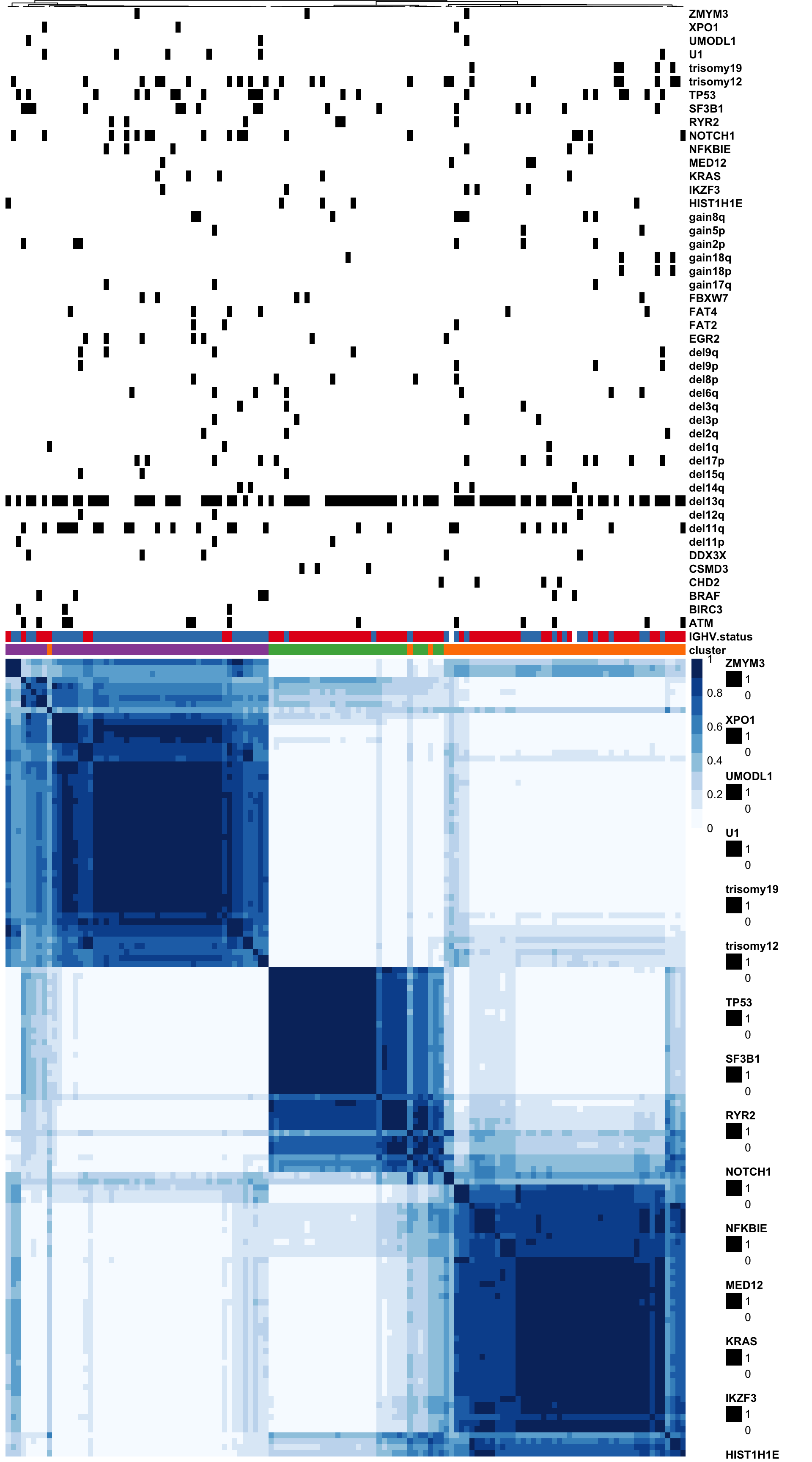
#dev.off()C1 and C3 groups are predominately M-CLL samples
table(clusterTab$cluster, clusterTab$IGHV.status)
      M  U
  C1 30  2
  C2  8 42
  C3 31 17
plotTab <- clusterTab %>%
filter(!is.na(IGHV.status)) %>%
group_by(cluster, IGHV.status) %>%
summarise(n=length(patientID))
ggplot(plotTab, aes(x=cluster,y=n, fill = IGHV.status)) +
geom_bar(stat="identity", postion = "stack") +
xlab("number of samples") +
scale_fill_manual(values = c(M = "#E41A1C", U = "#377EB8")) +
theme_my +
theme(legend.position = "bottom")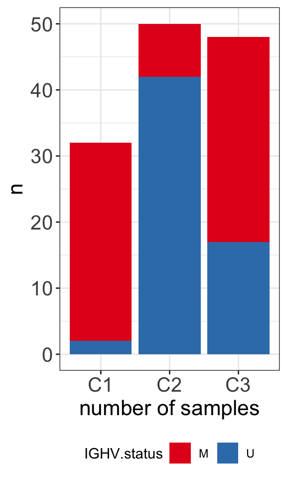
C1, C3 and C4 groups are predominately M-CLL samples
table(clusterTab$cluster, clusterTab$Mclust)
     HP IP LP
  C1 21  8  2
  C2  8  2 39
  C3 20 10 14
plotTab <- clusterTab %>%
filter(!is.na(Mclust)) %>%
group_by(cluster, Mclust) %>%
summarise(n=length(patientID))
ggplot(plotTab, aes(x=cluster,y=n, fill = Mclust)) +
geom_bar(stat="identity", postion = "stack") +
xlab("number of samples") +
#scale_fill_manual(values = c(M = "#E41A1C", U = "#377EB8")) +
theme_my +
theme(legend.position = "bottom")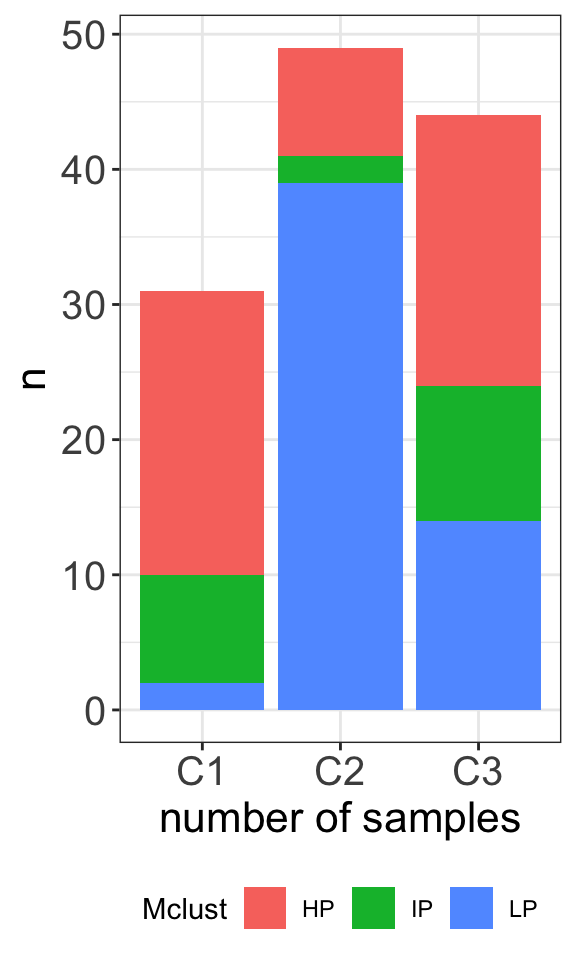
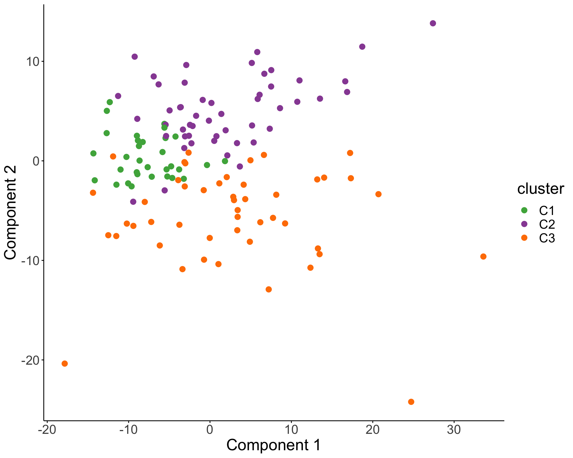
PCA visualization
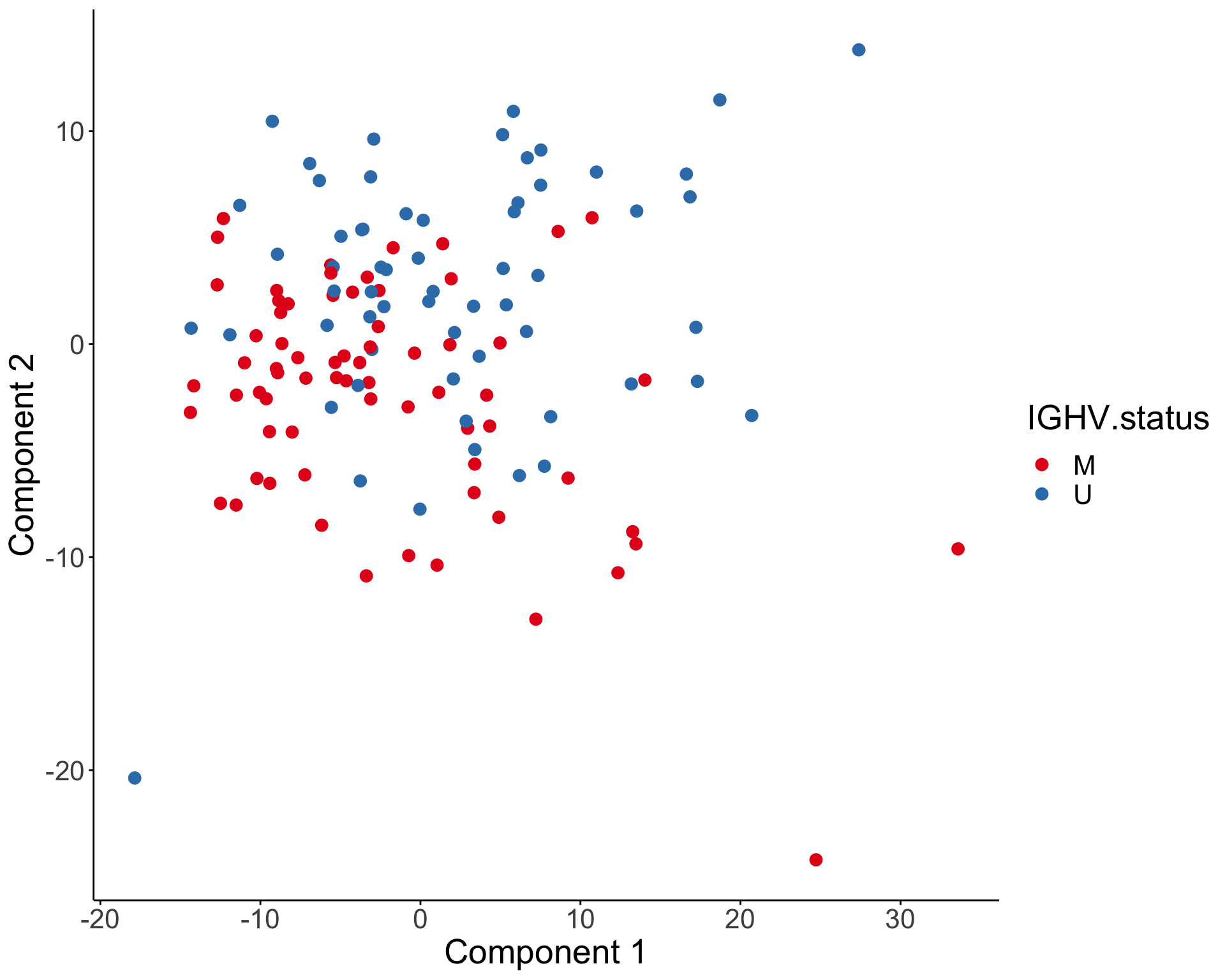
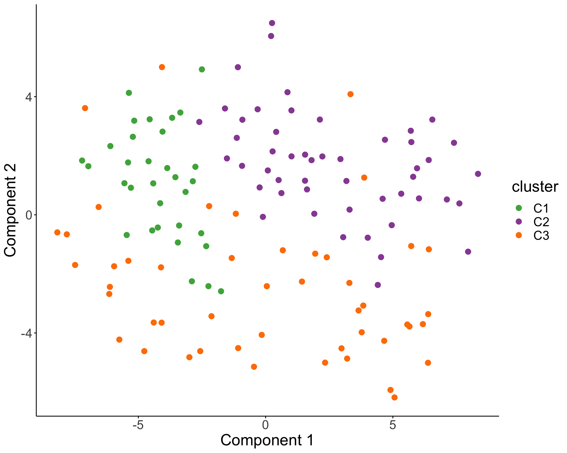
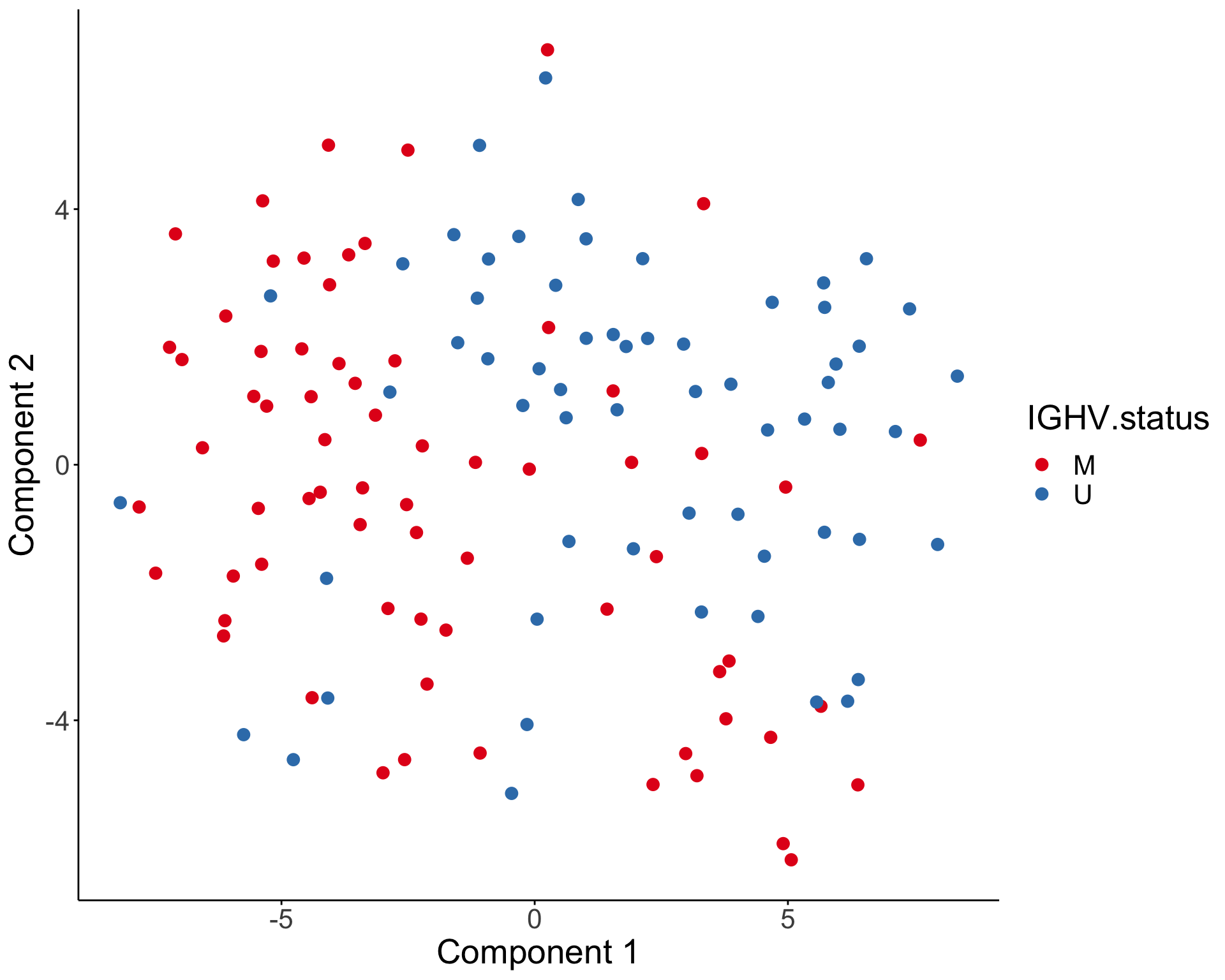
T-SNE visualization
Association with clinical outcomes (TTT and OS)
(Only M-CLL samples clustered as C1 and C3 groups are included)
load("../../var/survival_190516.RData")
testTab <- clusterTab %>% left_join(survT, by = "sampleID") %>%
  filter(!cluster%in% "C2", IGHV.status %in% "M")
Function for cox regression
com <- function(response, time, endpoint, scale =FALSE) {

  if (scale) {
    #calculate z-score
    response <- (response - mean(response, na.rm = TRUE))/sd(response, na.rm=TRUE)
  }
  surv <- coxph(Surv(time, endpoint) ~ response)


  tibble(p = summary(surv)[[7]][,5],
         HR = summary(surv)[[7]][,2],
         lower = summary(surv)[[8]][,3],
         higher = summary(surv)[[8]][,4])
}
Cox regression results
TTT
com(factor(testTab$cluster), testTab$TTT, testTab$treatedAfter)# A tibble: 1 × 4
p HR lower higher
<dbl> <dbl> <dbl> <dbl>
1 0.217 0.534 0.197 1.45OS
com(factor(testTab$cluster), testTab$OS, testTab$died)# A tibble: 1 × 4
p HR lower higher
<dbl> <dbl> <dbl> <dbl>
1 0.686 1.45 0.241 8.66Kaplan-Meier plots
Function for KM plot
formatNum <- function(i, limit = 0.01, digits =1, format="e") {
  r <- sapply(i, function(n) {
    if (n < limit) {
      formatC(n, digits = digits, format = format)
    } else {
      format(n, digits = digits)
    }
  })
  return(r)
}

theme_half <- ggplot2::theme_bw() + ggplot2::theme(axis.text = ggplot2::element_text(size=15),
                                 axis.title = ggplot2::element_text(size=16),
                                 axis.line = ggplot2::element_line(size=0.8),
                                 panel.border = ggplot2::element_blank(),
                                 axis.ticks = ggplot2::element_line(size=1.5),
                                 plot.title = ggplot2::element_text(size = 16, hjust =0.5, face="bold"),
                                 panel.grid.major = ggplot2::element_blank(),
                                 panel.grid.minor = ggplot2::element_blank())

km <- function(response, time, endpoint, titlePlot = "KM plot", pval = NULL,
               stat = "median", maxTime =NULL, showP = TRUE, showTable = FALSE,
               ylab = "Fraction", xlab = "Time (years)",
               table_ratio = c(0.7,0.3), yLabelAdjust = 0) {

  colList <- c("#BC3C29FF","#0072B5FF","#E18727FF","#20854EFF","#7876B1FF","#6F99ADFF","#FFDC91FF","#EE4C97FF")

  #function for km plot
  survS <- tibble(time = time,
                  endpoint = endpoint)

  if (!is.null(maxTime))
    survS <- mutate(survS, endpoint = ifelse(time > maxTime, FALSE, endpoint),
                    time = ifelse(time > maxTime, maxTime, time))

  if (stat == "maxstat") {
    ms <- maxstat.test(Surv(time, endpoint)  ~ response,
                       data = survS,
                       smethod = "LogRank",
                       minprop = 0.2,
                       maxprop = 0.8,
                       alpha = NULL)

    survS$group <- factor(ifelse(response >= ms$estimate, "high", "low"))
    p <- com(survS$group, survS$time, survS$endpoint)$p

  } else if (stat == "median") {
    med <- median(response, na.rm = TRUE)
    survS$group <- factor(ifelse(response >= med, "high", "low"))
    p <- com(survS$group, survS$time, survS$endpoint)$p

  } else if (stat == "binary") {
    survS$group <- factor(response)
    if (nlevels(survS$group) > 2) {
      sdf <- survdiff(Surv(survS$time,survS$endpoint) ~ survS$group)
      p <- 1 - pchisq(sdf$chisq, length(sdf$n) - 1)
    } else {
      p <- com(survS$group, survS$time, survS$endpoint)$p
    }
  }

  if (is.null(pval)) {
    if(p< 1e-16) {
      pAnno <- bquote(italic("P")~"< 1e-16")
    } else {
      pval <- formatNum(p, digits = 1)
      pAnno <- bquote(italic("P")~"="~.(pval))
    }

  } else {
     pval <- formatNum(pval, digits = 1)
     pAnno <- bquote(italic("P")~"="~.(pval))
  }

  if (!showP) pAnno <- ""

  colListNew <- colList[-4] #remove green
  colorPal <- colListNew[1:length(unique(survS$group))]
  p <- ggsurvplot(survfit(Surv(time, endpoint) ~ group, data = survS),
                  data = survS, pval = FALSE,  conf.int = FALSE, palette = colorPal,
                  legend = ifelse(showTable, "none","top"),
                  ylab = "Fraction", xlab = "Time (years)", title = titlePlot,
                  pval.coord = c(0,0.1), risk.table = showTable, legend.labs = sort(unique(survS$group)),
                  ggtheme = theme_half + theme(plot.title = element_text(hjust =0.5),
                                               panel.border = element_blank(),
                                               axis.title.y = element_text(vjust =yLabelAdjust)))
  if (!showTable) {
    p <- p$plot + annotate("text",label=pAnno, x = 0.1, y=0.1, hjust =0, size =5)
    return(p)
  } else {
    #construct a gtable
    pp <- p$plot + annotate("text",label=pAnno, x = 0.1, y=0.1, hjust =0, size=5)
    pt <- p$table + ylab("") + xlab("") + theme(plot.title = element_text(hjust=0, size =10))
    p <- plot_grid(pp,pt, rel_heights = table_ratio, nrow =2, align = "v")
    return(p)
  }
}
TTT
km(testTab$cluster, testTab$TTT, testTab$treatedAfter, "cluster VS TTT", stat = "binary", showTable = TRUE)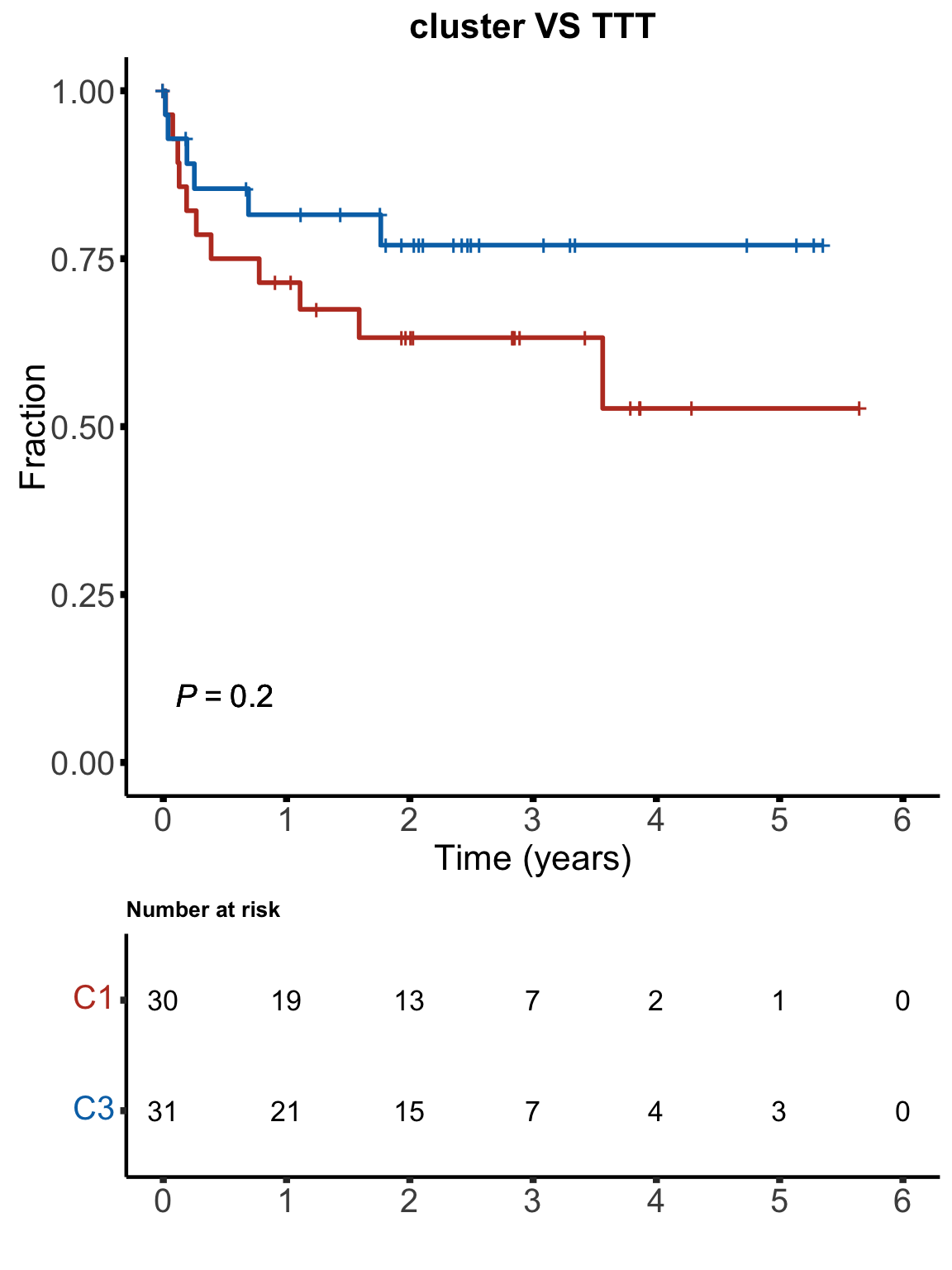
OS
km(testTab$cluster, testTab$OS, testTab$died, "cluster VS OS", stat = "binary", showTable = TRUE)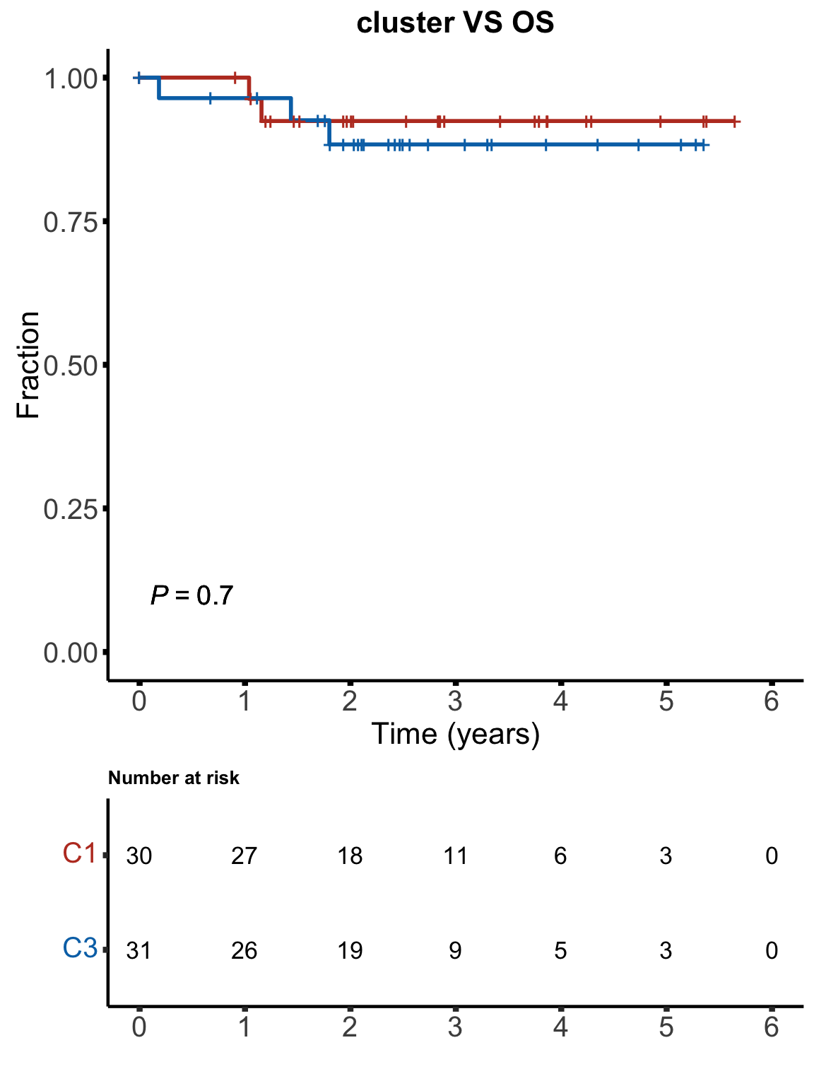
Baseline ATP levels after 48 hours
Baseline ATP is the ATP level in the control wells after 48 hours of culture. It can be regarded as a baseline viability of the cells.
load("~/CLLproject_jlu/var/newEMBL_20210129.RData")
basalATP <- emblNew %>% filter(type == "neg") %>%
  group_by(patID) %>% summarise(ATPcount = median(val, na.rm=TRUE))
All samples
testTab <- clusterTab %>%
  left_join(basalATP, by = c(patientID = "patID"))
#t.test(log(ATPcount) ~ cluster, testTab, var.equal=TRUE)

ggplot(testTab, aes(x=cluster, y=log(ATPcount))) +
  geom_boxplot(outlier.shape = NA, width=0.3) +
  ggbeeswarm::geom_quasirandom(aes(col = cluster)) +
  scale_color_manual(values = annoCol$cluster) +
  ylab("baseline ATP") +
  theme_my + theme(legend.position = "none")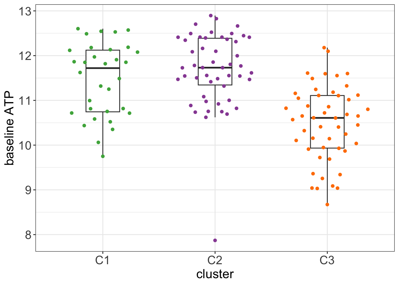
Stratified by IGHV
testTab <- clusterTab %>%
  left_join(basalATP, by = c(patientID = "patID")) %>%
  filter(!is.na(IGHV.status))
#t.test(log(ATPcount) ~ cluster, testTab, var.equal=TRUE)

ggplot(testTab, aes(x=cluster, y=log(ATPcount))) +
  geom_boxplot(outlier.shape = NA, width=0.3) +
  ggbeeswarm::geom_quasirandom(aes(col = cluster)) +
  scale_color_manual(values = annoCol$cluster) +
  ylab("baseline ATP") +
  facet_wrap(~IGHV.status) +
  theme_my + theme(legend.position = "none")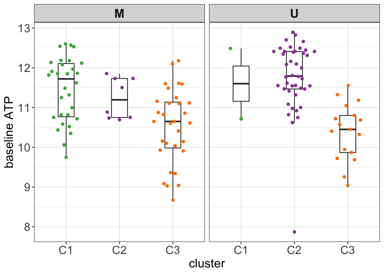
Whether it correlates with CLL-PD?
load("~/CLLproject_jlu/analysis/CLLsubgroup/facTab_CPSatLeast3New.RData")
testTab <- clusterTab %>%
  mutate(CLLPD = facTab[match(patientID, facTab$patID),]$factor)

#t.test(CLLPD ~ cluster, testTab, var.equal=TRUE)

ggplot(testTab, aes(x=cluster, y=CLLPD)) +
  geom_boxplot(outlier.shape = NA, width=0.3) +
  ggbeeswarm::geom_quasirandom(aes(col = cluster)) +
  scale_color_manual(values = annoCol$cluster) +
  ylab("CLL-PD") +
  theme_my + theme(legend.position = "none")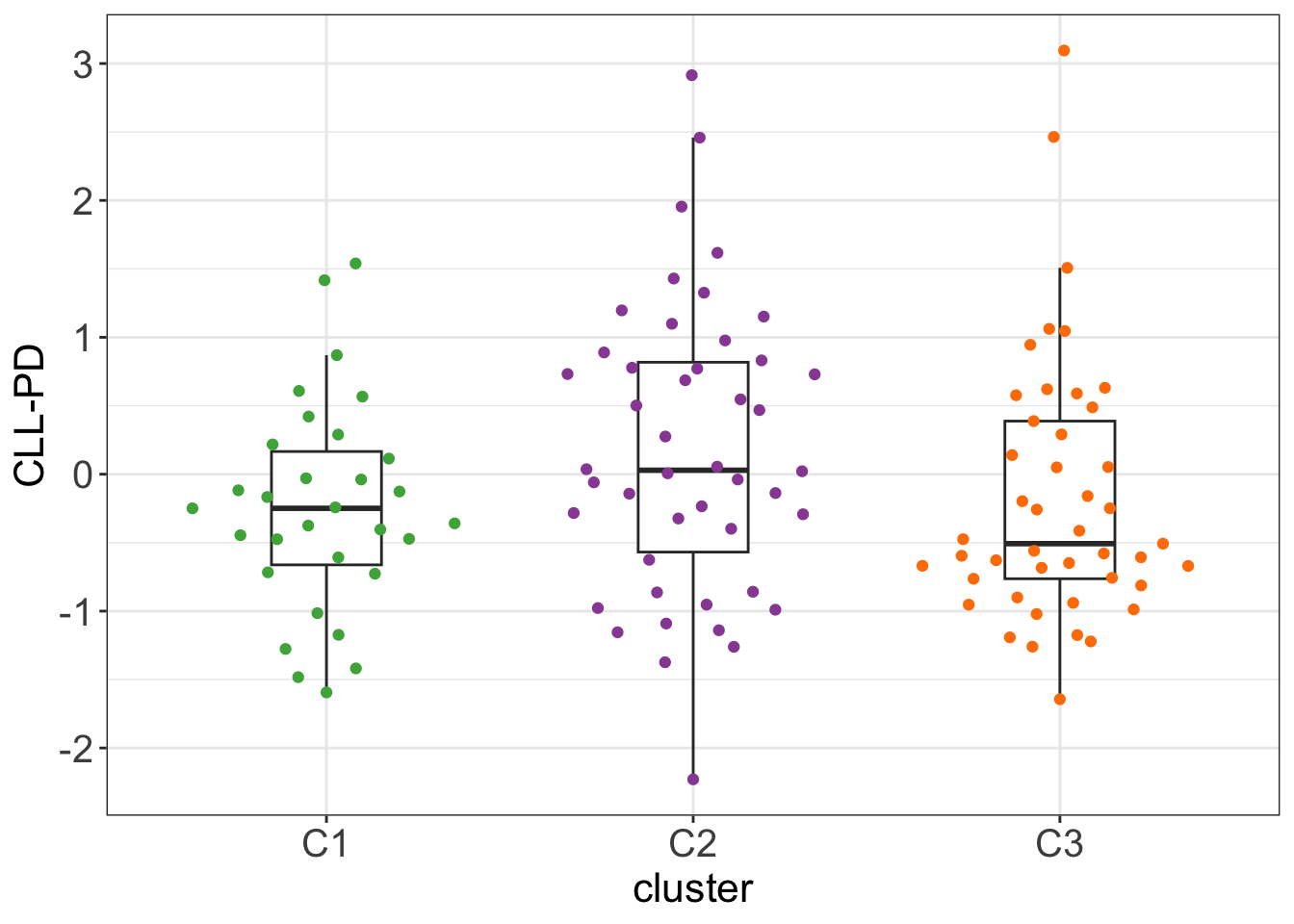
Stratified by IGHV status
testTab <- clusterTab %>%
  mutate(CLLPD = facTab[match(patientID, facTab$patID),]$factor) %>%
  filter(!is.na(IGHV.status))

#t.test(CLLPD ~ cluster, testTab, var.equal=TRUE)

ggplot(testTab, aes(x=cluster, y=CLLPD)) +
  geom_boxplot(outlier.shape = NA, width=0.3) +
  ggbeeswarm::geom_quasirandom(aes(col = cluster)) +
  scale_color_manual(values = annoCol$cluster) +
  ylab("CLL-PD") +
  facet_wrap(~IGHV.status) +
  theme_my + theme(legend.position = "none")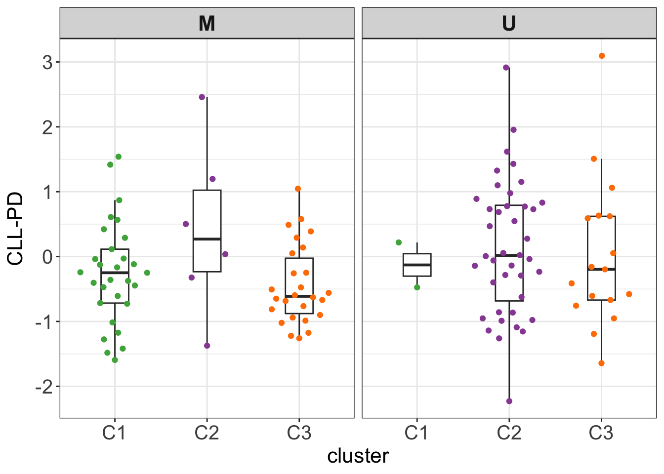
Identify drug that associate with the 4 groups (independent of their IGHV status)
ANOVA test
testTabAll <- screenData %>%
  mutate(IGHV.status = patMeta[match(patientID, patMeta$Patient.ID),]$IGHV.status) %>%
  filter(diagnosis %in% "CLL", !is.na(IGHV.status)) %>% #only CLL
  distinct(patientID, Drug, .keep_all = TRUE) %>%
  select(patientID, Drug, viab.auc) %>%
  dplyr::rename(viab = viab.auc) %>%
  left_join(clusterTab, by = "patientID")

resTab <- testTabAll %>% group_by(Drug) %>% nest() %>%
  mutate(m=map(data, ~car::Anova(lm(viab~ IGHV.status + cluster, .,)))) %>%
  mutate(res = map(m, broom::tidy)) %>%
  unnest(res) %>% ungroup() %>%
  filter(term == "cluster") %>%
  select(Drug, p.value) %>%
  mutate(p.adj = p.adjust(p.value, method = "BH")) %>%
  arrange(p.value)

resTab.sig <- filter(resTab, p.adj < 0.1)
Boxplot of top 18 associated drugs
drugList <- resTab$Drug[1:18]

plotTabBox <- filter(testTabAll, Drug %in% drugList) %>%
  mutate(pathway = drugAnno[match(Drug, drugAnno$drugName),]$pathway) %>%
  mutate(drugPath = sprintf("%s\n(%s)", Drug, pathway))

ggplot(plotTabBox, aes(x=cluster, y = viab)) +
  geom_boxplot(outlier.shape = NA, aes(fill = cluster)) +
  ggbeeswarm::geom_quasirandom(aes(col=IGHV.status)) +
  facet_wrap(~drugPath, scale ="free_x", ncol=3) +
  scale_fill_manual(values = annoCol$cluster) +
  scale_color_manual(values = annoCol$IGHV.status) +
  theme_my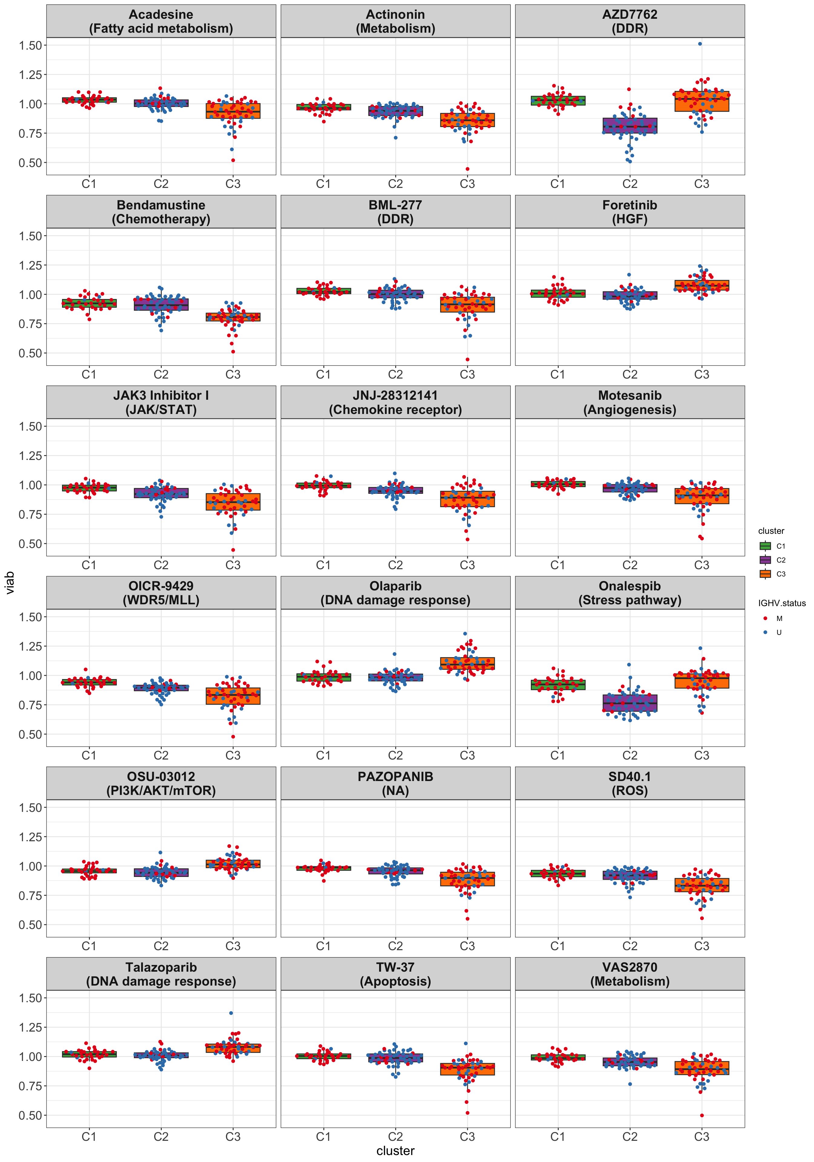
Heatmap visualization of drug passed 10% FDR
viabMatScale <- jyluMisc::mscale(viabMatImp[rownames(viabMatImp) %in% resTab.sig$Drug,], censor =5)
viabMatScale <- viabMatScale[,arrange(clusterTab,cluster)$patientID]

pheatmap(viabMatScale, scale="none", clustering_method = "ward.D2", clustering_distance_cols = "correlation",
         cluster_cols = FALSE,
         annotation_col = colAnnoAlt,
         annotation_colors = annoCol,
         color = colorRampPalette(c("red","white","blue"))(100), show_colnames = FALSE)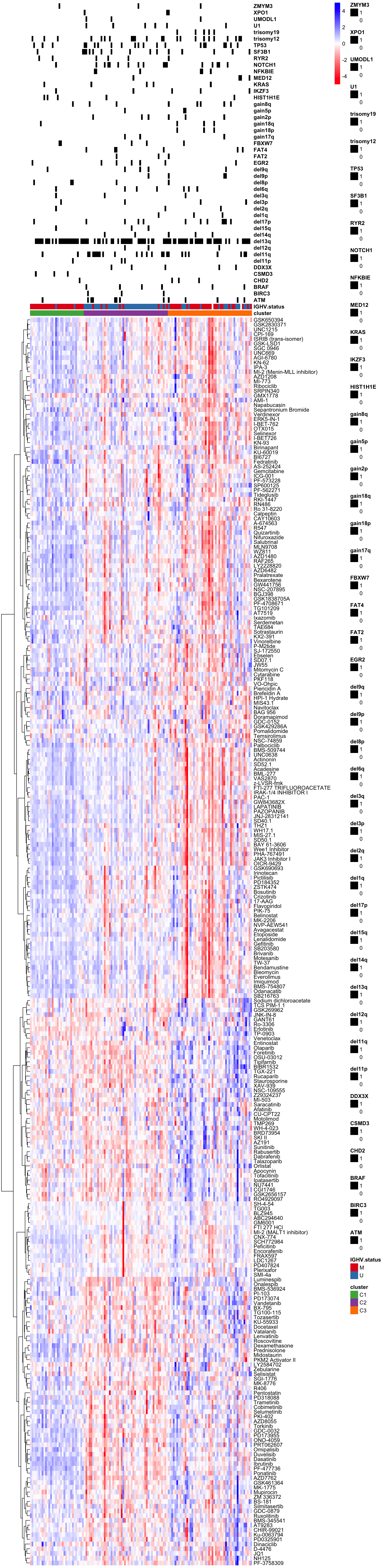
Characterize the drug response phenotypes of C1 and C3 subgroup within M-CLL samples
In this part, I want to answer the question how C1 and C3 subgroups are different in terms of drug response profile. As samples in C1 and C3 group are primarily M-CLL samples, in the analysis below, only M-CLL samples will be considered.
Identify drugs that show differential responses between C1 and C3 in M-CLL samples
testTabAll <- screenData %>%
  mutate(IGHV.status = patMeta[match(patientID, patMeta$Patient.ID),]$IGHV.status) %>%
  filter(diagnosis %in% "CLL", !is.na(IGHV.status)) %>% #only CLL
  distinct(patientID, Drug, .keep_all = TRUE) %>%
  select(patientID, Drug, viab.auc) %>%
  dplyr::rename(viab = viab.auc) %>%
  left_join(clusterTab, by = "patientID") %>%
  filter(cluster != "C4")

testTab <- testTabAll %>%
  filter(cluster %in% c("C1","C3"),
         IGHV.status %in% "M",
         !is.na(viab)) %>%
  mutate(cluster =factor(cluster, levels = c("C1","C3")))

#at least five samples if each cluster for each drug, this is because for some drugs the AUC could not be fitted
drugFilt <- group_by(testTab, cluster, Drug) %>%
  summarise(n = length(!is.na(viab))) %>%
  pivot_wider(names_from = cluster, values_from = n) %>%
  filter(C1>=5 & C3>=5)

testTab <- filter(testTab, Drug %in% drugFilt$Drug)
resTab <- testTab %>% group_by(Drug) %>% nest() %>%
mutate(m=map(data, ~t.test(viab~cluster, ., var.equal=TRUE))) %>%
mutate(res = map(m, broom::tidy)) %>%
unnest(res) %>% ungroup() %>%
select(Drug, estimate, p.value, estimate1, estimate2) %>%
mutate(p.adj = p.adjust(p.value, method = "BH"), log2FC = log2(estimate2/estimate1)) %>%
arrange(p.value) %>%
mutate(pathway = drugAnno[match(Drug, drugAnno$drugName),]$pathway) %>%
mutate(drugPath = sprintf("%s (%s)", Drug, pathway))
resTab.sig <- resTab %>% filter(p.adj < 0.1)Volcano plot
plotTabVol <- resTab %>%
  mutate(direction = case_when(p.adj > 0.01 ~ "n.s.",
                               p.adj < 0.01 & log2FC <0 ~ "sensitive in C3",
                               p.adj < 0.01 & log2FC >0 ~ "resistent in C3"))

#label top 20 drugs judged by pvalue
topDrug <- arrange(resTab, p.value)$Drug[1:20]
plotTabVol <- mutate(plotTabVol, drugLabel = ifelse(Drug %in% topDrug, as.character(drugPath), ""))

ggplot(plotTabVol, aes(y=-log10(p.adj), x= log2FC)) +
  geom_point(aes(col = direction)) +
  geom_hline(yintercept = 2, linetype ="dashed") +
  ggrepel::geom_text_repel(aes(label = drugLabel),max.overlaps=100) +
  scale_color_manual(values = c(n.s. = "grey50", `sensitive in C3` = "blue", `resistent in C3` = "red")) +
  #xlim(-0.5,0.5) +
  ggtitle("Drug sensitivity between C1 and C3\n(within M-CLL samples)") +
  theme_my +
  theme(plot.title = element_text(hjust=0.5, size=15, face ="bold"))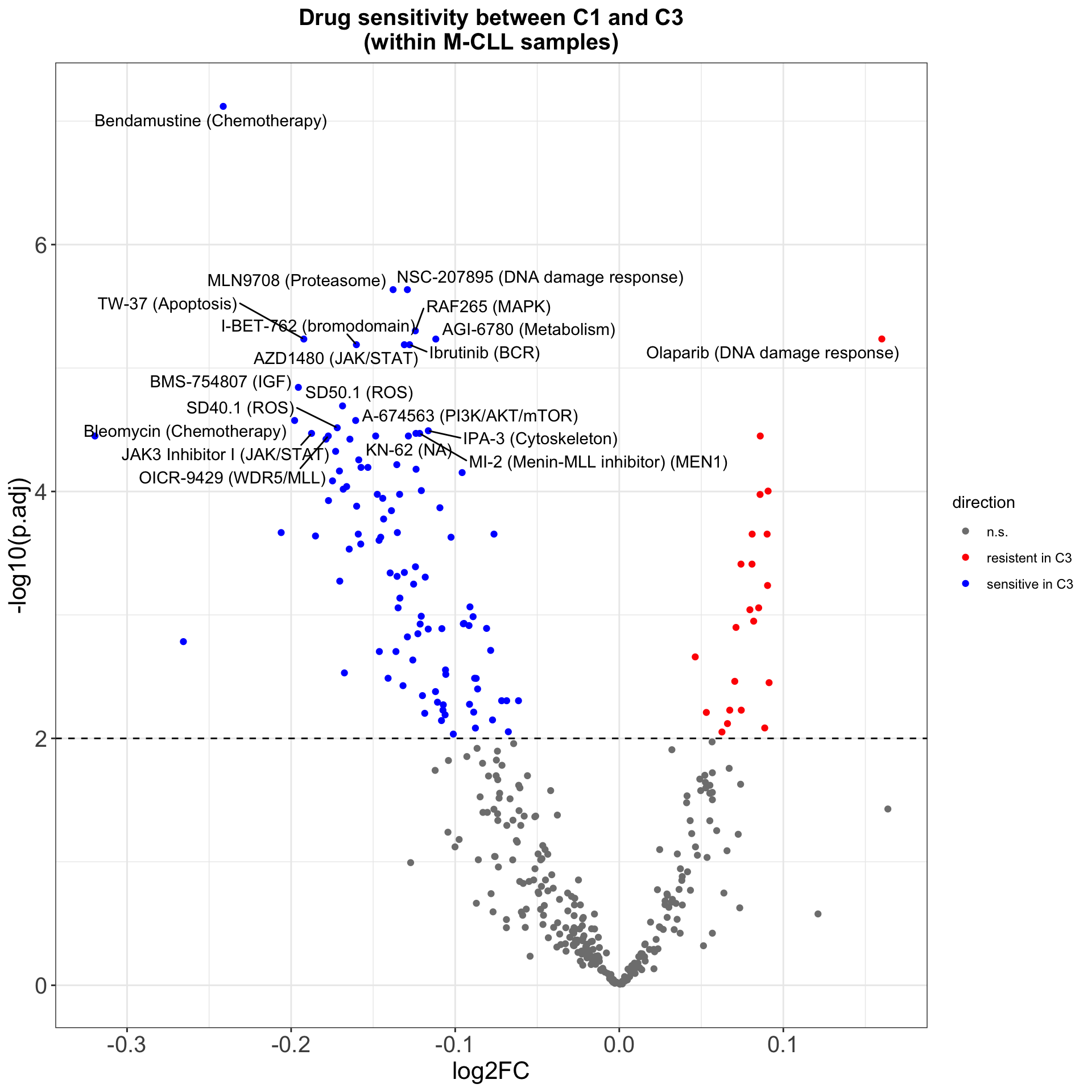
ggsave("volcano.png", height = 5, width = 6)Drug with 1% FDR and abs(log2FC) > 0.5 are labeled
A list of all drugs associated with C1/C3 subgroups
10% FDR cut-off is used
resTab %>% filter(p.adj < 0.1) %>%
  mutate_if(is.numeric, formatC, digits=2) %>%
  select(-drugPath) %>%
  DT::datatable()
Visualization with viability matrix of associated drugs
viabMatScale <- jyluMisc::mscale(viabMatImp[rownames(viabMatImp) %in% resTab.sig$Drug, colnames(viabMatImp) %in% testTab$patientID], censor =5)
viabMatScale <- viabMatScale[,unique(arrange(testTab,cluster)$patientID)]

pheatmap(viabMatScale, scale="none", clustering_method = "ward.D2", clustering_distance_cols = "correlation",
         cluster_cols = FALSE,
         annotation_col = colAnnoAlt,
         annotation_colors = annoCol,
         color = colorRampPalette(c("red","white","blue"))(100), show_colnames = FALSE)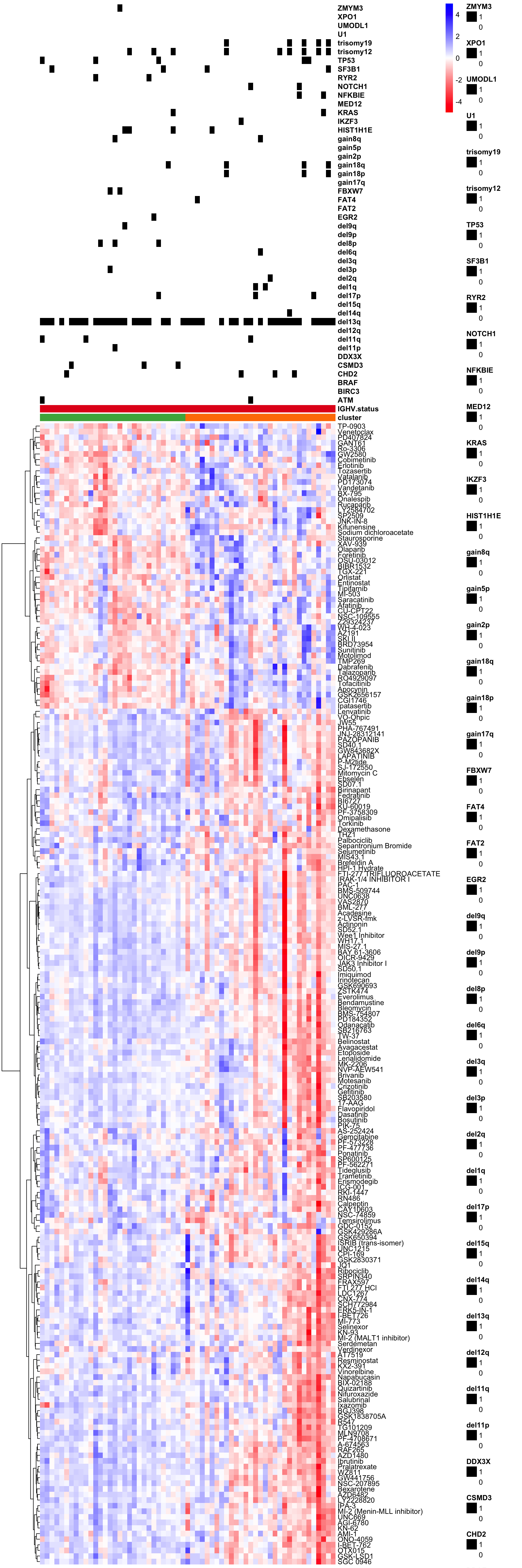
Boxplots
Only M-CLL samples that belong to C1 and C3 group
drugList <- filter(plotTabVol, drugLabel != "")$Drug
plotTabBox <- filter(testTab, Drug %in% drugList) %>%
  mutate(pathway = drugAnno[match(Drug, drugAnno$drugName),]$pathway) %>%
  mutate(drugPath = sprintf("%s\n(%s)", Drug, pathway))
ggplot(plotTabBox, aes(x=cluster, y = viab)) +
  geom_boxplot(outlier.shape = NA, aes(fill = cluster)) + ggbeeswarm::geom_quasirandom() +
  facet_wrap(~drugPath) +
  theme_my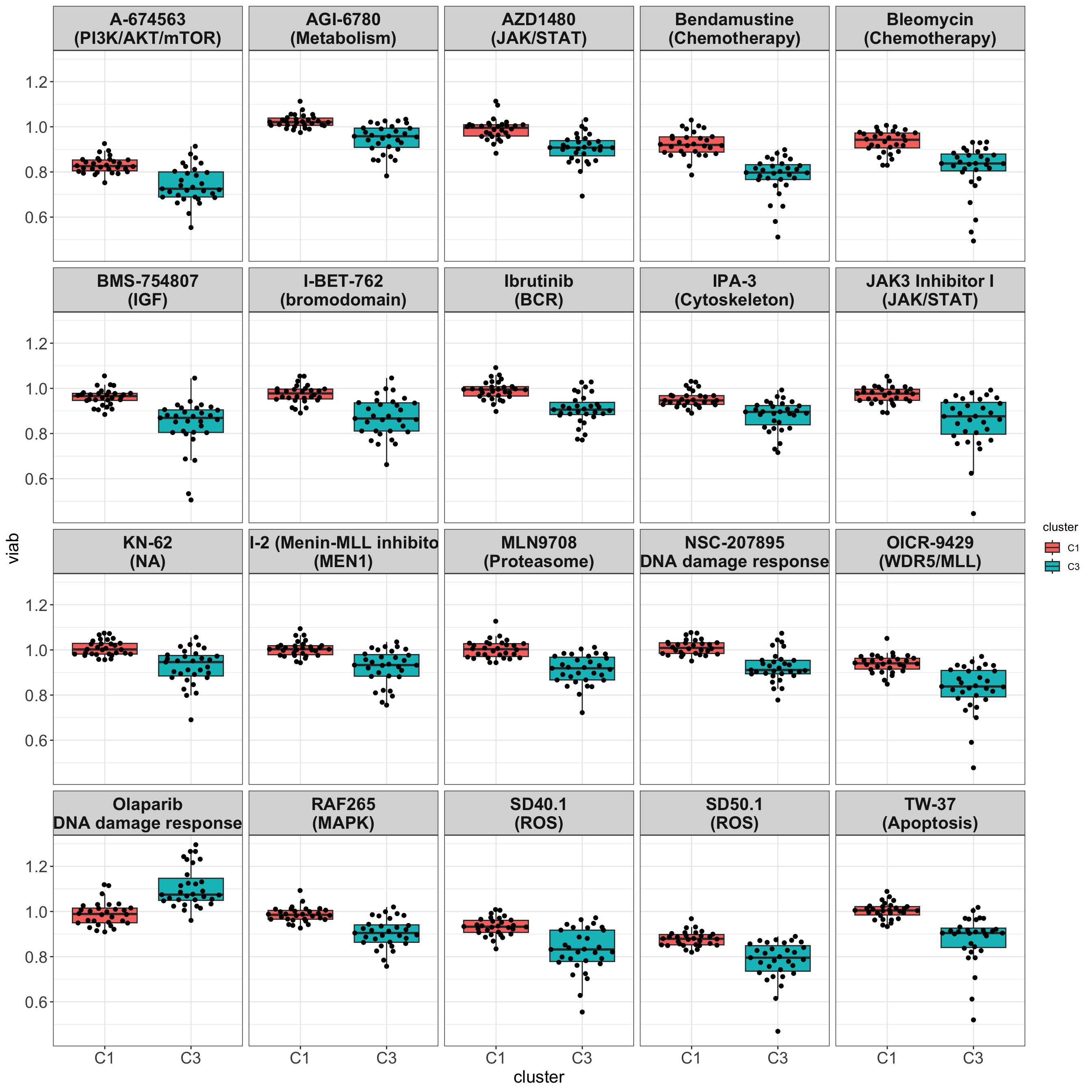
All samples and colored by their IGHV status
drugList <- filter(plotTabVol, drugLabel != "")$Drug
plotTabBox <- filter(testTabAll, Drug %in% drugList, !is.na(IGHV.status)) %>%
  mutate(pathway = drugAnno[match(Drug, drugAnno$drugName),]$pathway) %>%
  mutate(drugPath = sprintf("%s\n(%s)", Drug, pathway))
ggplot(plotTabBox, aes(x=cluster, y = viab)) +
  geom_boxplot(outlier.shape = NA) +
  ggbeeswarm::geom_quasirandom(aes(col= IGHV.status)) +
  scale_color_manual(values = c(M = "#E41A1C", U = "#377EB8")) +
  facet_wrap(~drugPath, ncol=4) +
  ylab("Viability (AUC)") + xlab("Clusters") +
  theme_my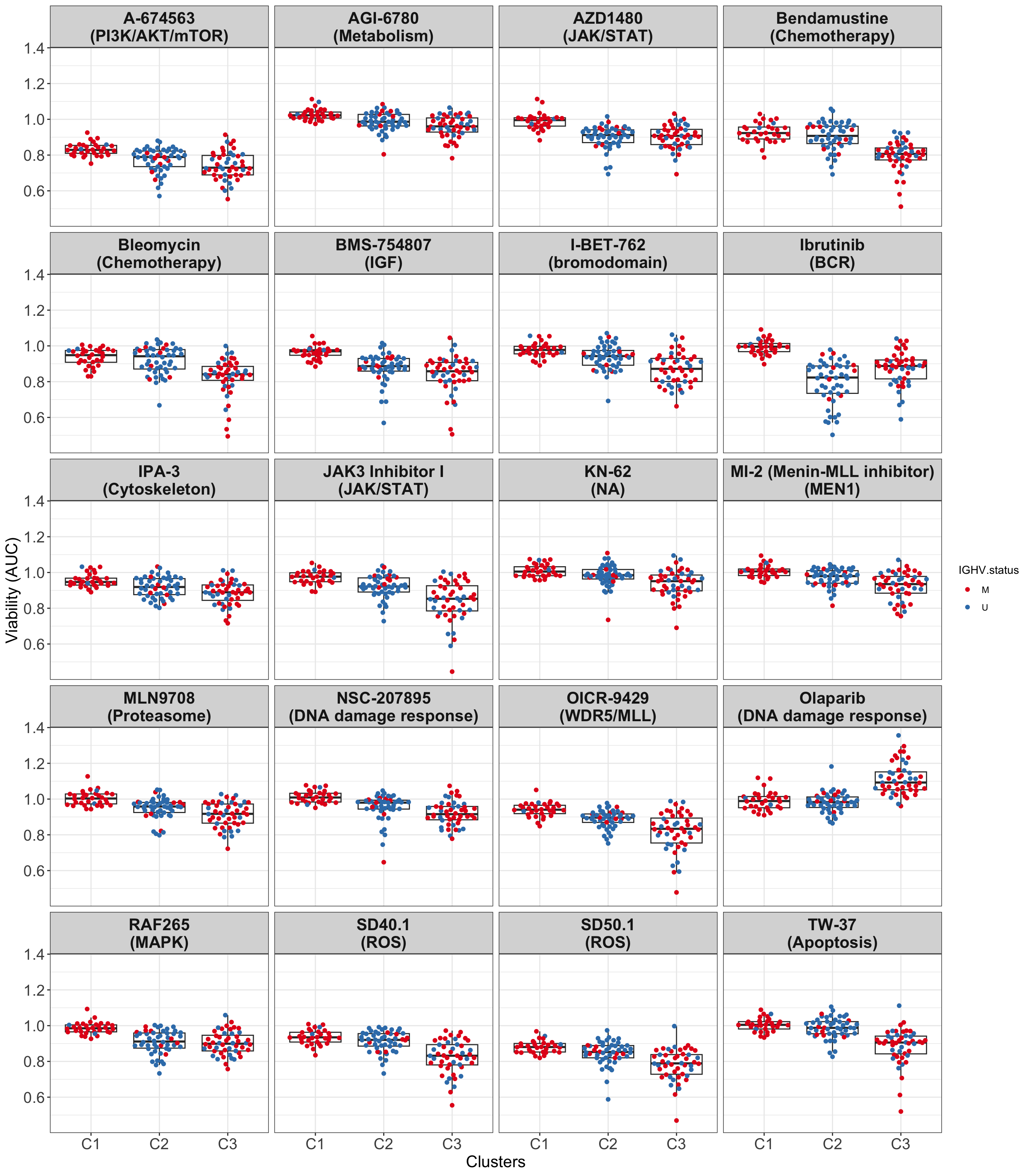
#ggsave("boxplot_AUC.png", height = 6, width = 12)It can be seen that for many drugs, the difference between C1 and C3 groups are even larger than between C2 (U-CLL) and C1 or C2 and C3.
Distribution of target (all drugs passed 1% FDR will be considered)
More resistant
Over-representation test
classAnno <- distinct(screenData, Drug, class)
targetAnno <- select(drugAnno, drugName, target,pathway) %>%
  left_join(classAnno, by = c(drugName = "Drug"))
resTabSig <- resTab %>%
  filter(p.adj <0.01, log2FC > 0) %>%
  left_join(targetAnno, by = c(Drug = "drugName")) %>%
  mutate(pathway=pathway.x)
drugAll <- filter(targetAnno, drugName %in% resTab$Drug) %>%
mutate(ifSig = drugName %in% resTabSig$Drug)
enrichTab <- lapply(unique(resTabSig$class), function(n) {
drugTest <- filter(drugAll, !is.na(class)) %>%
mutate(ifGroup = class %in% n)
tt <- table(drugTest$ifGroup, drugTest$ifSig)
res <- fisher.test(tt, alternative = "greater")
data.frame(class = n, p = res$p.value)
}) %>% bind_rows() %>% arrange(p)
head(enrichTab) class p
1 Differentiating /Epigenetic modifier 0.1263263
2 Hedgehog inhibitor 0.2525528
3 Immunomodulatory 0.4094913
4 Other 0.5539799
5 Metabolic modifier 0.6760808
6 Kinase inhibitor 0.7108863enrichTab <- lapply(na.omit(unique(resTabSig$pathway)), function(n) {
drugTest <- filter(drugAll, !is.na(pathway)) %>%
mutate(ifGroup = pathway %in% n)
tt <- table(drugTest$ifGroup, drugTest$ifSig)
res <- fisher.test(tt, alternative = "greater")
data.frame(class = n, p = res$p.value)
}) %>% bind_rows() %>% arrange(p)
head(enrichTab) class p
1 DNA damage response 0.02357063
2 MEN1 0.10816387
3 TAM 0.15797386
4 Notch 0.15797386
5 Cytokine receptor 0.20512733
6 Hedgehog 0.24975922More sensitive
Over-representation test
classAnno <- distinct(screenData, Drug, class)
targetAnno <- select(drugAnno, drugName, target, pathway) %>%
  left_join(classAnno, by = c(drugName = "Drug"))
resTabSig <- resTab %>%
  filter(p.adj <0.01, log2FC < 0 ) %>%
  left_join(targetAnno, by = c(Drug = "drugName")) %>%
  mutate(pathway = pathway.x)
drugAll <- filter(targetAnno, drugName %in% resTab$Drug) %>%
mutate(ifSig = drugName %in% resTabSig$Drug)
enrichTab <- lapply(unique(resTabSig$class), function(n) {
drugTest <- filter(drugAll, !is.na(class)) %>%
mutate(ifGroup = class %in% n)
tt <- table(drugTest$ifGroup, drugTest$ifSig)
res <- fisher.test(tt, alternative = "greater")
data.frame(class = n, p = res$p.value)
}) %>% bind_rows() %>% arrange(p)
head(enrichTab) class p
1 ROS 0.005741289
2 Apoptotic modulator 0.131103238
3 Protease/Proteosome inhibitor 0.337665079
4 Conventional Chemo 0.437261739
5 Immunomodulatory 0.451706812
6 Differentiating /Epigenetic modifier 0.582142339enrichTab <- lapply(na.omit(unique(resTabSig$pathway)), function(n) {
drugTest <- filter(drugAll, !is.na(pathway)) %>%
mutate(ifGroup = pathway %in% n)
tt <- table(drugTest$ifGroup, drugTest$ifSig)
res <- fisher.test(tt, alternative = "greater")
data.frame(class = n, p = res$p.value)
}) %>% bind_rows() %>%
arrange(p)
head(enrichTab) class p
1 ROS 0.005266872
2 Cell adhesion 0.069470759
3 JAK/STAT 0.131238159
4 Apoptosis 0.177914772
5 bromodomain 0.191555042
6 Vitamin 0.264550265General toxicity and group
meanViabTab <-screenData %>%
  group_by(Drug) %>% summarise(meanViab = mean(viab.auc, na.rm=TRUE)) %>%
  left_join(resTab, by = "Drug") %>%
  mutate(dir = case_when(p.adj <0.01 & log2FC >0 ~ "resistant in C3",
                         p.adj <0.01 & log2FC < 0 ~ "sensitive in C3",
                         TRUE~ "not associated"))
car::Anova(lm(meanViab ~ dir, meanViabTab))
Anova Table (Type II tests)
Response: meanViab
Sum Sq Df F value Pr(>F)
dir 0.0750 2 3.8476 0.02215 *
Residuals 3.7807 388
---
Signif. codes: 0 '***' 0.001 '**' 0.01 '*' 0.05 '.' 0.1 ' ' 1ggplot(meanViabTab, aes(x=dir, y=meanViab)) +
geom_boxplot() + geom_point() +
theme_my +
ylab("mean viability among all samples") + xlab("")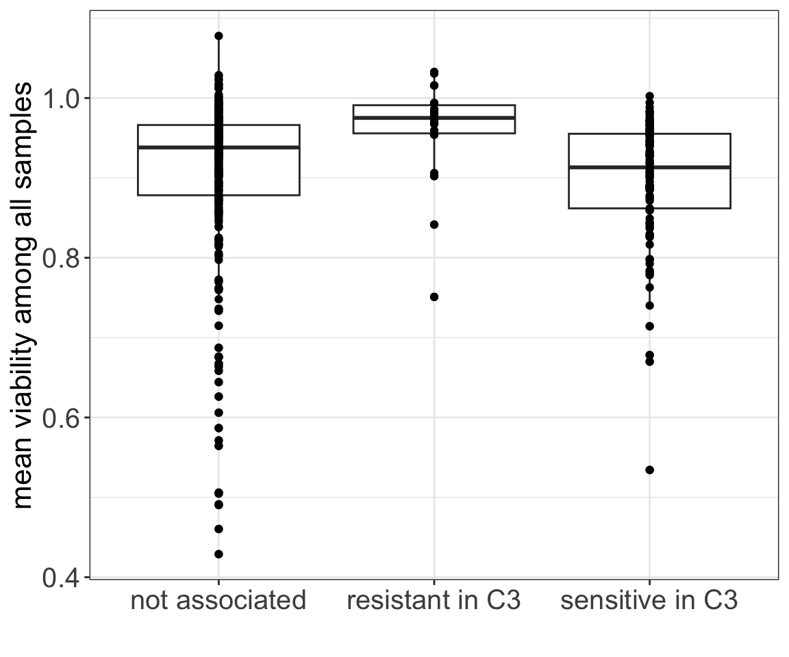
ggsave("toxivity_box.png", width = 5, height = 4)Multi-omics characterization of C1 and C3 groups
In this part, I want to answer the questions that why samples in C1 and C3 groups response differently to those above drugs. In order to explain this, I will look at some of the omics data we have.
Does it correlate with previous identified mTOR group?
All CLLs
drugGroup <- read_csv("~/CLLproject_jlu/data/expressionAnalysis/selNEW.csv") %>%
  select(`...1`, group) %>% dplyr::rename(patID = `...1`) %>%
  mutate(cluster = clusterTab[match(patID, clusterTab$patientID),]$cluster) %>%
  filter(!is.na(cluster))

table(drugGroup$group, drugGroup$cluster)
       C1 C2 C3
  BTK   0 14  1
  MEK   2  4  2
  mTOR  2  1  6
  none 10  7 10
Within M-CLLs
drugGroup <- mutate(drugGroup, IGHV = patMeta[match(patID, patMeta$Patient.ID),]$IGHV.status) %>%
  filter(cluster %in% c("C1","C3"), IGHV %in% "M")
table(drugGroup$group, drugGroup$cluster)
       C1 C3
  MEK   2  1
  mTOR  2  5
  none  9  4
The C1 and C3 groups identified from EMBL2016 screen are not the same as drug sensitivity groups previously identified. Although the C1 group maybe related to the non-responder group. But C3 is not the mTOR group
plotEve <- filter(screenData, Drug %in% c("Everolimus","Rapamycin")) %>%
  group_by(Drug, patientID) %>% summarise(viab = mean(viab.auc)) %>%
  mutate(cluster = clusterTab[match(patientID, clusterTab$patientID),]$cluster,
         IGHV = patMeta[match(patientID, patMeta$Patient.ID),]$IGHV.status) %>%
  filter(cluster %in% c("C1","C3"), IGHV %in% "M")

ggplot(plotEve, aes(x=cluster, y = viab)) +
  geom_boxplot(width=0.3) +
  ggbeeswarm::geom_quasirandom(aes(col = cluster)) +
  scale_color_manual(values = annoCol$cluster) +
  facet_wrap(~Drug) +
  ylab("Viability (AUC)") +
  theme_my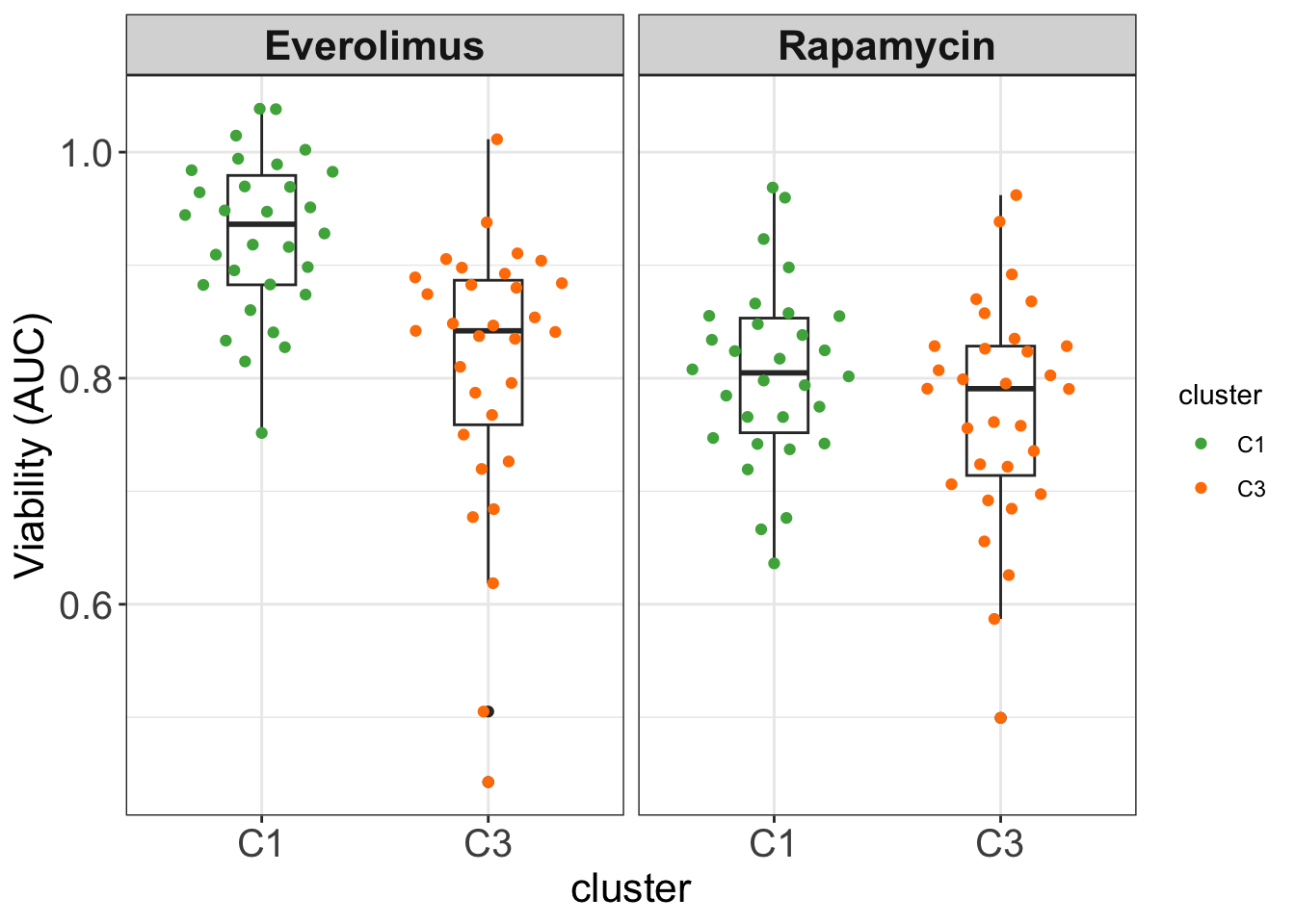
Correlations between genomics/demographics and C1/C3 groups
clusterAnno <- filter(clusterTab, cluster %in% c("C1","C3"), IGHV.status == "M") %>%
  mutate(pretreat = treatmentTab[match(sampleID, treatmentTab$sampleID),]$pretreat)
geneTab <- select(patMeta, Patient.ID, gender, Methylation_Cluster, del10p:U1) %>%
  dplyr::rename(sex = gender)
testTab <- select(clusterAnno, patientID, cluster, pretreat) %>%
  left_join(geneTab, by = c(patientID = "Patient.ID")) %>%
  mutate_all(as.character) %>%
  pivot_longer(!c(patientID, cluster))

sumTab <- group_by(testTab, name) %>%
  summarise(noNA = sum(!is.na(value)), numMut = sum(value %in% c("1","m","HP", "M"))) %>%
  filter(noNA > 40, numMut >=5)

testTab <- filter(testTab, name %in% sumTab$name)
resTab <- group_by(testTab, name) %>% nest() %>%
mutate(m=map(data, ~chisq.test(.$cluster, .$value))) %>%
mutate(res = map(m, broom::tidy)) %>%
unnest(res) %>%
select(name, p.value) %>%
arrange(p.value)
resTab# A tibble: 7 × 2
# Groups: name [7]
name p.value
<chr> <dbl>
1 trisomy19 0.0617
2 sex 0.370
3 trisomy12 0.504
4 TP53 0.969
5 del13q 1.00
6 pretreat 1.00
7 Methylation_Cluster 1 No significant associations can be identified, indicating the C1/C3 group is not driven by genomic, demographic or treatment. It can potentially be a new functional group
Transcriptomic characterization (baseline expression).
Differential gene expression between C1 and C3 groups
load("../../var/ddsrna_180717.RData")
dds$cluster <- factor(clusterAnno[match(dds$PatID, clusterAnno$patientID),]$cluster)
dds$CLLPD <- facTab[match(dds$PatID, facTab$patID),]$factor
dds$IGHV <- factor(patMeta[match(dds$PatID, patMeta$Patient.ID),]$IGHV.status)
ddsSub <- dds[,!is.na(dds$cluster)]
ddsSub <- ddsSub[rowMedians(counts(ddsSub, normalized = TRUE)) > 10,]
ddsSub <- ddsSub[rowData(ddsSub)$biotype %in% "protein_coding",]
ddsSub <- ddsSub[!rowData(ddsSub)$symbol %in% c("", NA)]
table(ddsSub$cluster)
C1 C3
30 28
library(DESeq2)
design(ddsSub) <- ~cluster
deRes <- DESeq(ddsSub)Table of differentially expressed genes (10% FDR)
resTab <- results(deRes, tidy = TRUE, name = "cluster_C3_vs_C1") %>%
  mutate(symbol = rowData(ddsSub[row,])$symbol) %>%
  arrange(pvalue)

resTab.sig <- filter(resTab, padj < 0.1) %>%
  mutate(symbol = factor(symbol, levels = symbol))
DT::datatable(resTab.sig %>% select(symbol, row, stat, pvalue, padj) %>%
                mutate_if(is.numeric, formatC, digits=2))
P-value histogram
hist(resTab$pvalue)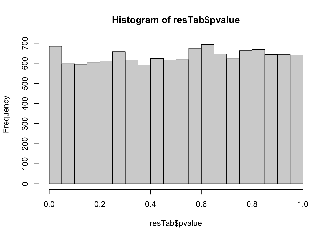
Boxplots of top 9 candidates based on p-value
plotTab <- counts(ddsSub, normalized = TRUE)[resTab.sig$row[1:9],] %>%
  as_tibble(rownames = "id") %>% pivot_longer(-id) %>%
  mutate(cluster = clusterAnno[match(name, clusterAnno$patientID),]$cluster) %>%
  left_join(resTab.sig, by = c(id = "row"))

ggplot(plotTab, aes(x=cluster, y=log10(value))) +
  geom_boxplot(outlier.shape = NA, width=0.3) +
  ggbeeswarm::geom_quasirandom(aes(col=cluster)) +
  facet_wrap(~symbol, scale ="free") +
  scale_color_manual(values = annoCol$cluster) +
  ylab("RNAseq count") +
  theme_my + theme(legend.position = "none")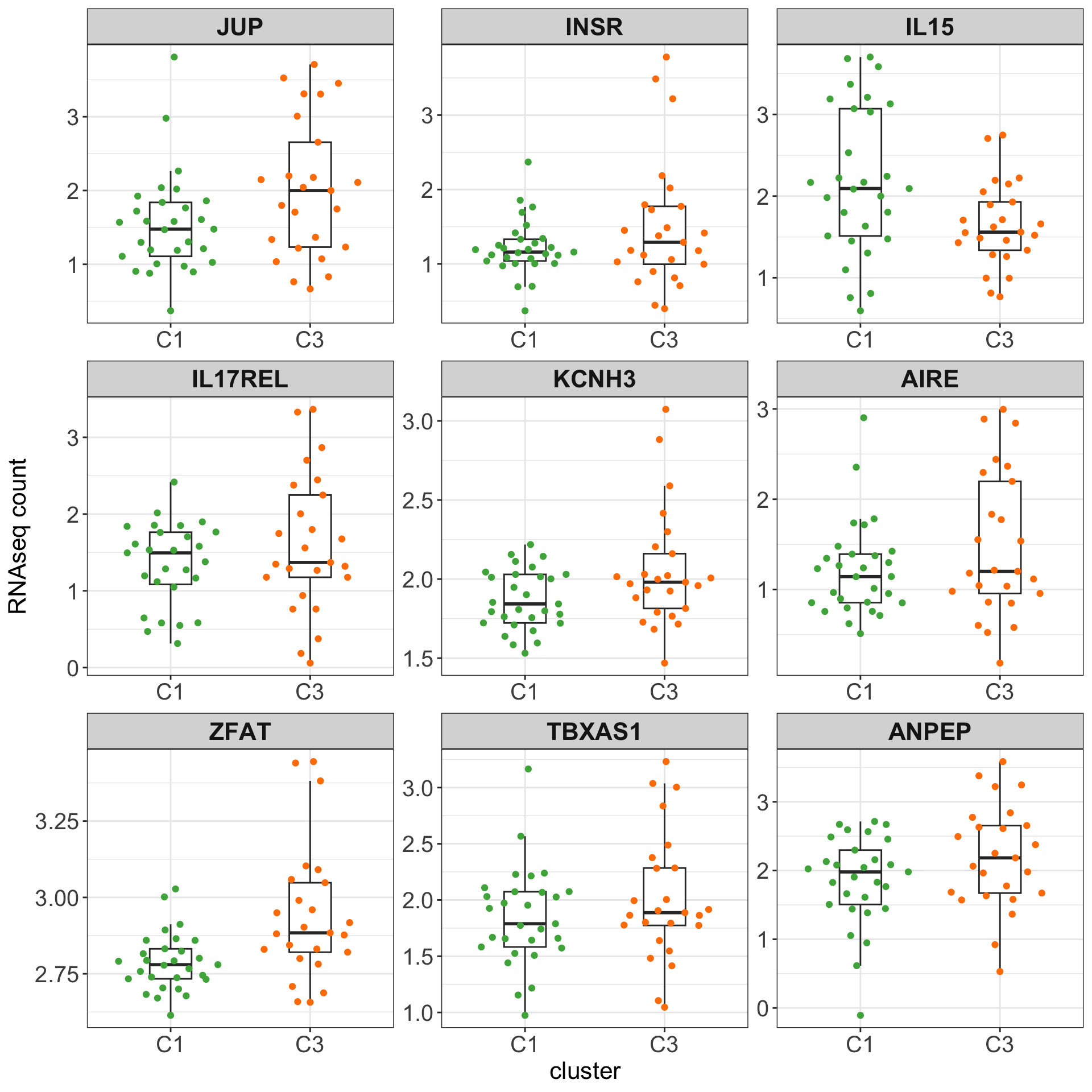
Pathway enrichment analysis
exprMat <- counts(ddsSub)
exprMat <- limma::voom(exprMat, lib.size = ddsSub$sizeFactor)$E
designMat <- model.matrix(~ddsSub$cluster)
Hallmark gene sets
(Raw p values < 0.05, no sets passed 10% FDR)
gmts <- list(H = "~/CLLproject_jlu/data/commonFiles/h.all.v6.2.symbols.gmt",
             KEGG = "~/CLLproject_jlu/data/commonFiles/c2.cp.kegg.v5.1.symbols.gmt")
enHallmark <- jyluMisc::runCamera(exprMat, designMat, gmts$H, id = rowData(ddsSub)$symbol,ifFDR = TRUE, pCut =0.25, plotTitle = "Cancer Hallmarks")
enHallmark$enrichPlot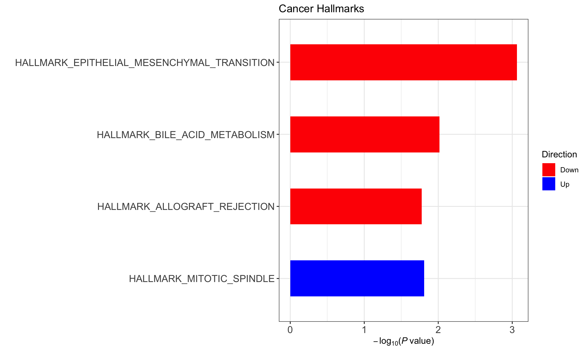
KEGG gene set
(Raw p values < 0.05, no sets passed 10% FDR)
gmts <- list(H = "~/CLLproject_jlu/data/commonFiles/h.all.v6.2.symbols.gmt",
             KEGG = "~/CLLproject_jlu/data/commonFiles/c2.cp.kegg.v5.1.symbols.gmt")
enHallmark <- jyluMisc::runCamera(exprMat, designMat, gmts$KEGG, id = rowData(ddsSub)$symbol,ifFDR = TRUE, pCut =0.1, plotTitle = "KEGG gene sets")
[1] "No sets passed the criteria"enHallmark$enrichPlotNULLTranscriptomic characterization (expression after cultured in DMSO for 48h).
Differential gene expression between C1 and C3 groups
load("~/CLLproject_jlu/analysis/drugSeq/ddsAll.RData")
dds <- ddsAll[,ddsAll$treatment =="DMSO"]
dds$cluster <- factor(clusterAnno[match(dds$patID, clusterAnno$patientID),]$cluster)
dds$CLLPD <- facTab[match(dds$patID, facTab$patID),]$factor
dds$IGHV <- factor(patMeta[match(dds$patID, patMeta$Patient.ID),]$IGHV.status)
colnames(dds) <- dds$patID
ddsSub <- dds[,!is.na(dds$cluster)]
table(ddsSub$cluster)
C1 C3
10  9
ddsSub <- ddsSub[rowMedians(counts(ddsSub, normalized = TRUE)) > 10,]
ddsSub <- ddsSub[rowData(ddsSub)$biotype %in% "protein_coding",]
ddsSub <- ddsSub[!rowData(ddsSub)$symbol %in% c("", NA)]
sds <- genefilter::rowSds(counts(ddsSub, normalized = TRUE))
ddsSub <- ddsSub[sds > genefilter::shorth(sds),]library(DESeq2)
design(ddsSub) <- ~cluster
deRes <- DESeq(ddsSub, betaPrior = TRUE)Table of differentially expressed genes (10% FDR)
resTab <- results(deRes, tidy = TRUE) %>%
  mutate(symbol = rowData(ddsSub[row,])$symbol) %>%
  arrange(pvalue)

resTab.sig <- filter(resTab, pvalue < 0.01) %>%
  mutate(symbol = factor(symbol, levels = symbol))
DT::datatable(resTab.sig %>% select(symbol, row, stat, pvalue, padj) %>%
                mutate_if(is.numeric, formatC, digits=2))
P-value histogram
hist(resTab$pvalue)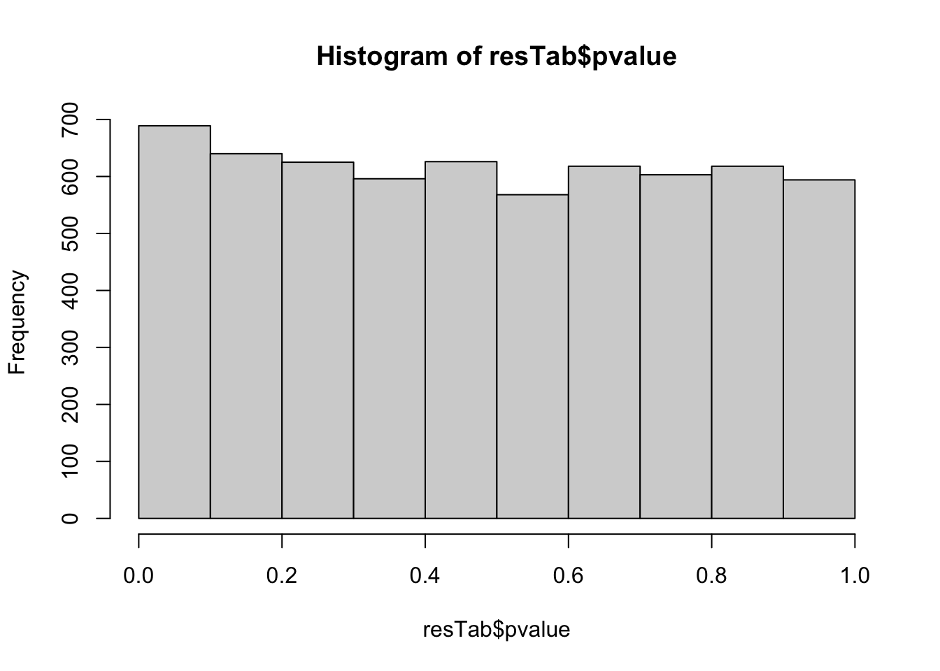
Boxplots of top 9 candidates based on p-value
plotTab <- counts(ddsSub, normalized = TRUE)[resTab.sig$row[1:9],] %>%
  as_tibble(rownames = "id") %>% pivot_longer(-id) %>%
  mutate(cluster = clusterAnno[match(name, clusterAnno$patientID),]$cluster) %>%
  left_join(resTab.sig, by = c(id = "row"))

ggplot(plotTab, aes(x=cluster, y=log10(value))) +
  geom_boxplot(outlier.shape = NA, width=0.3) +
  ggbeeswarm::geom_quasirandom(aes(col=cluster)) +
  facet_wrap(~symbol, scale ="free") +
  scale_color_manual(values = annoCol$cluster) +
  ylab("RNAseq count") +
  theme_my + theme(legend.position = "none")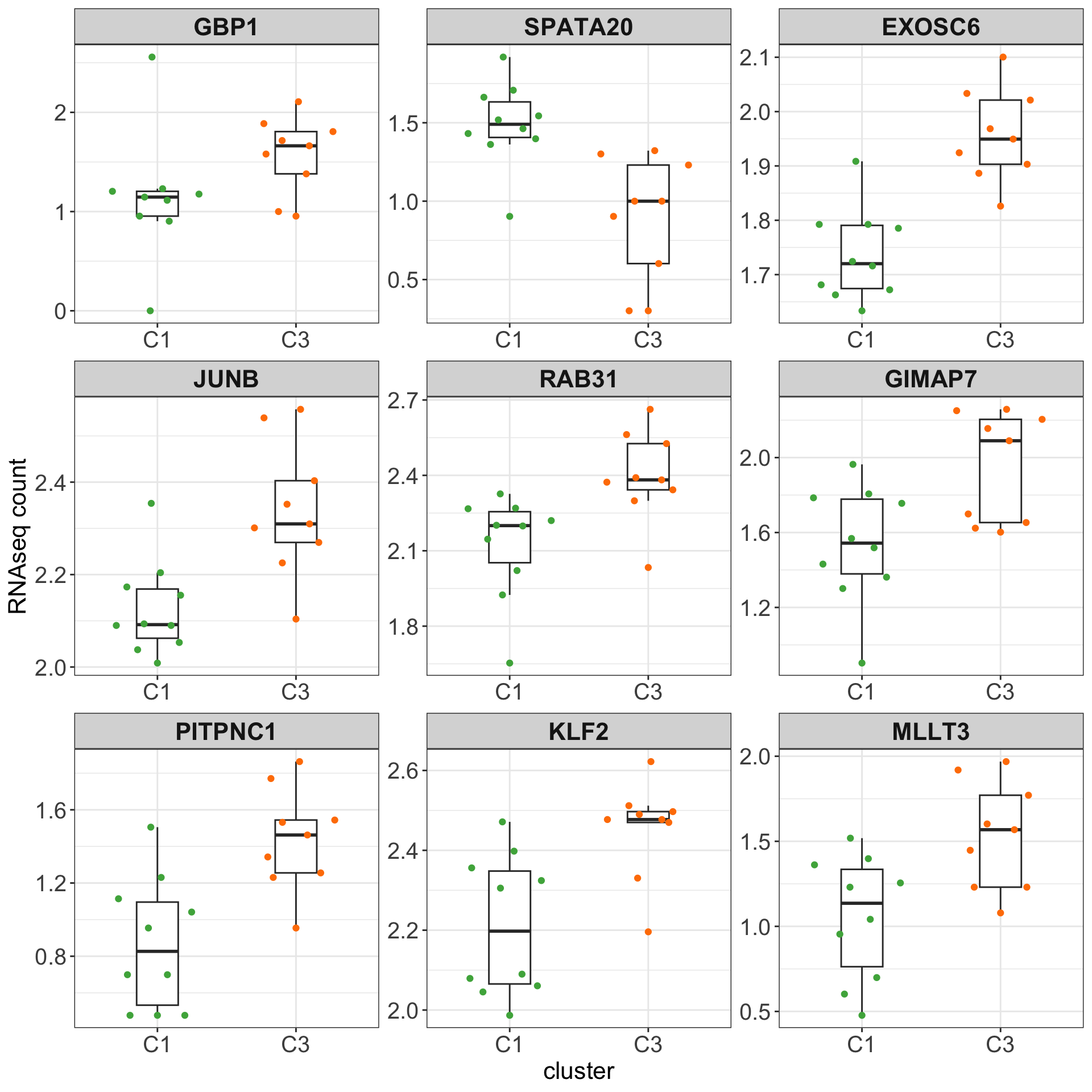
Pathway enrichment analysis
exprMat <- counts(ddsSub)
exprMat <- limma::voom(exprMat, lib.size = ddsSub$sizeFactor)$E
designMat <- model.matrix(~ddsSub$cluster)
Hallmark gene sets
(Raw p values < 0.05, no sets passed 10% FDR)
gmts <- list(H = "~/CLLproject_jlu/data/commonFiles/h.all.v6.2.symbols.gmt",
             KEGG = "~/CLLproject_jlu/data/commonFiles/c2.cp.kegg.v5.1.symbols.gmt")
enHallmark <- jyluMisc::runCamera(exprMat, designMat, gmts$H, id = rowData(ddsSub)$symbol,ifFDR = TRUE, pCut =0.25, plotTitle = "Cancer Hallmarks")
enHallmark$enrichPlot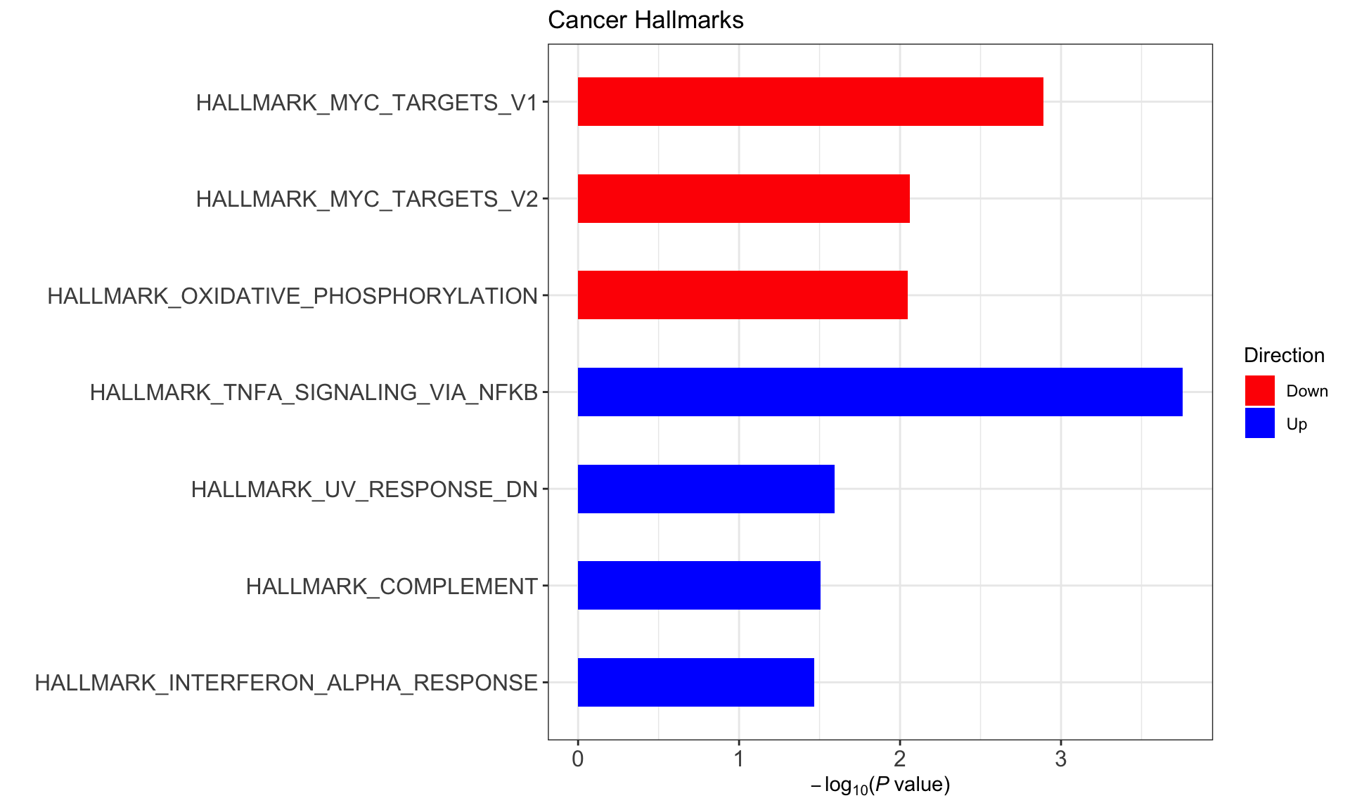
KEGG gene set
(Raw p values < 0.05, no sets passed 10% FDR)
gmts <- list(H = "~/CLLproject_jlu/data/commonFiles/h.all.v6.2.symbols.gmt",
             KEGG = "~/CLLproject_jlu/data/commonFiles/c2.cp.kegg.v5.1.symbols.gmt")
enHallmark <- jyluMisc::runCamera(exprMat, designMat, gmts$KEGG, id = rowData(ddsSub)$symbol,ifFDR = TRUE, pCut =0.1, plotTitle = "KEGG gene sets")
enHallmark$enrichPlot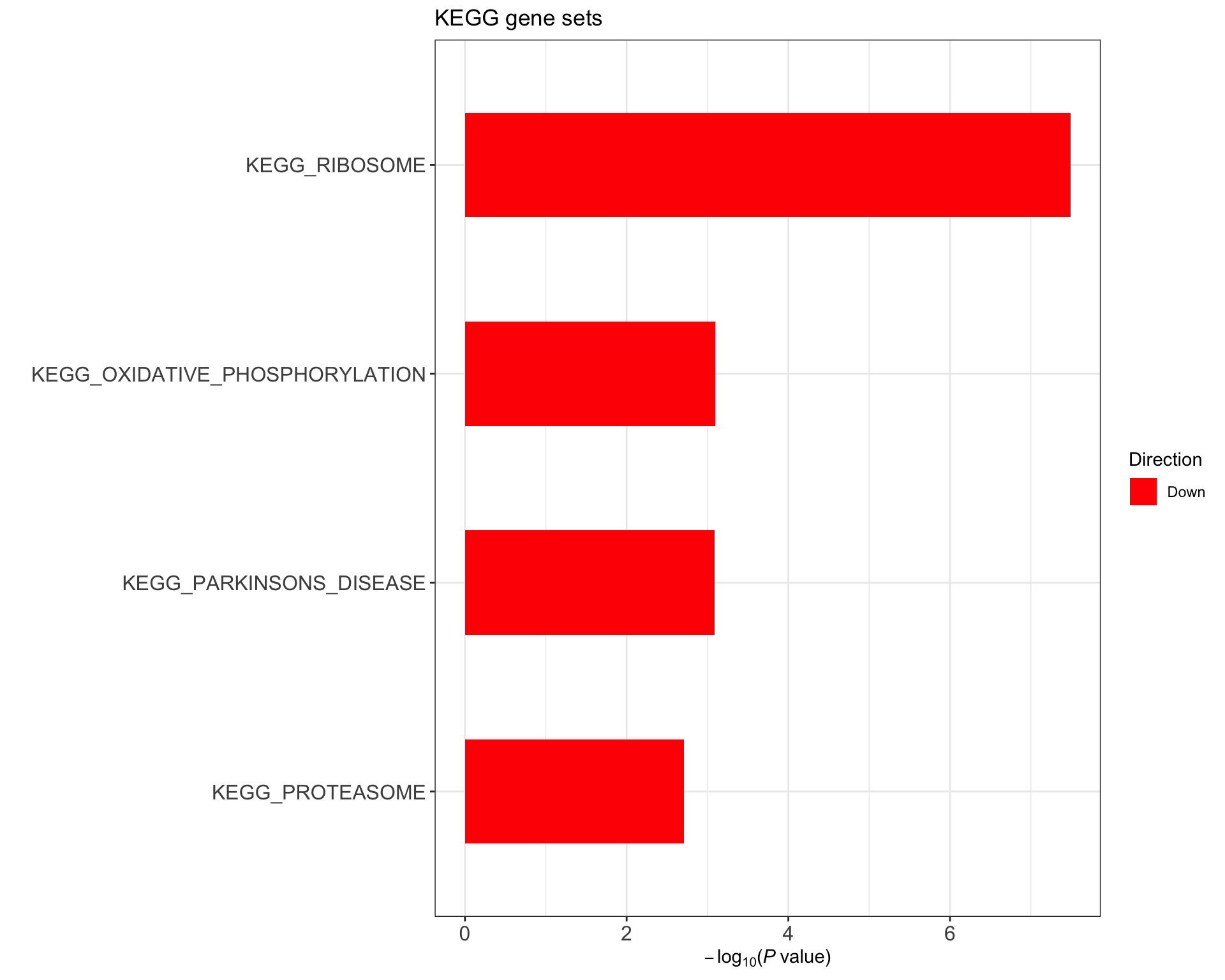
Differential expression at protein levels
load("../../var/proteomic_LUMOS_batch13.RData")
protCLL$patID <- colnames(protCLL)
protCLL$cluster <- factor(clusterAnno[match(protCLL$patID, clusterAnno$patientID),]$cluster)
protCLL$CLLPD <- facTab[match(protCLL$patID, facTab$patID),]$factor
protCLL$IGHV <- factor(patMeta[match(protCLL$patID, patMeta$Patient.ID),]$IGHV.status)
protSub <- protCLL[,!is.na(protCLL$cluster)]

table(protCLL$cluster)
C1 C3
10 16
Differential expression
library(proDA)
designMat <- data.frame(row.names = protSub$patID,
                         cluster = protSub$cluster,
                         batch = protSub$batch)

protMat <- assays(protSub)[["count"]]

fit <- proDA(protMat, design = ~ .,
             col_data = designMat)

resTab <- test_diff(fit, "clusterC3") %>%
  dplyr::rename(id = name, logFC = diff, t=t_statistic,
                pvalue = pval, padj = adj_pval) %>%
  mutate(symbol = rowData(protCLL[id,])$hgnc_symbol) %>%
  select(symbol, id, logFC, t, pvalue, padj, n_obs) %>%
  arrange(pvalue) %>%
  as_tibble()
Tables of candiates with P value < 0.01
(none passed 10% FDR)
resTab.sig <- filter(resTab, pvalue < 0.01) %>%
  mutate(symbol = factor(symbol, levels = symbol))
DT::datatable(resTab.sig %>% select(symbol, logFC, pvalue, padj) %>%
                mutate_if(is.numeric, formatC, digits=2))
P-value histogram
hist(resTab$pvalue)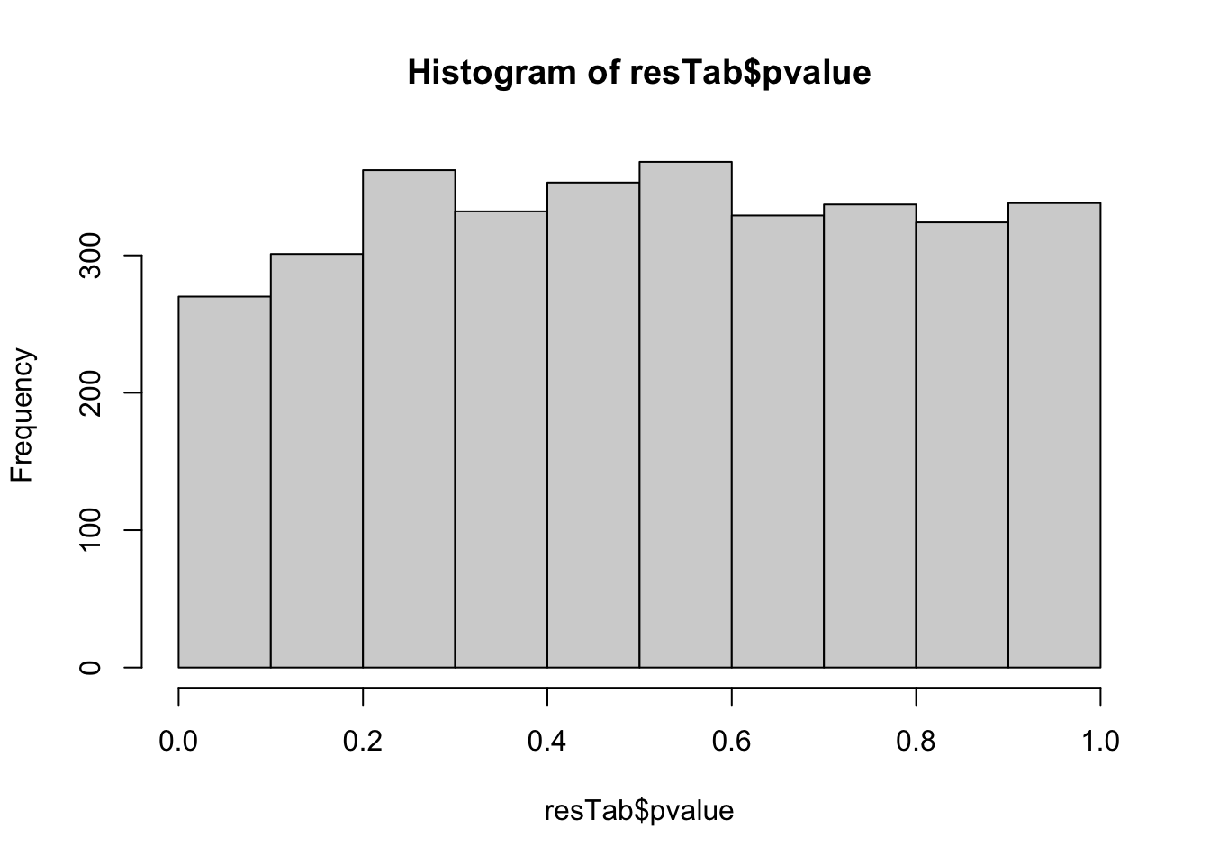
Boxplots of top 9 candidates
plotTab <- assays(protSub)[["log2Norm_combat"]][resTab.sig$id[1:9],] %>%
  as_tibble(rownames = "id") %>% pivot_longer(-id) %>%
  mutate(cluster = clusterAnno[match(name, clusterAnno$patientID),]$cluster) %>%
  left_join(resTab.sig, by = "id")

ggplot(plotTab, aes(x=cluster, y=log10(value))) +
  geom_boxplot(outlier.shape = NA, width=0.3) +
  ggbeeswarm::geom_quasirandom(aes(col = cluster)) +
  scale_color_manual(values = annoCol$cluster) +
  facet_wrap(~symbol, scale ="free") +
  theme_my + theme(legend.position = "none")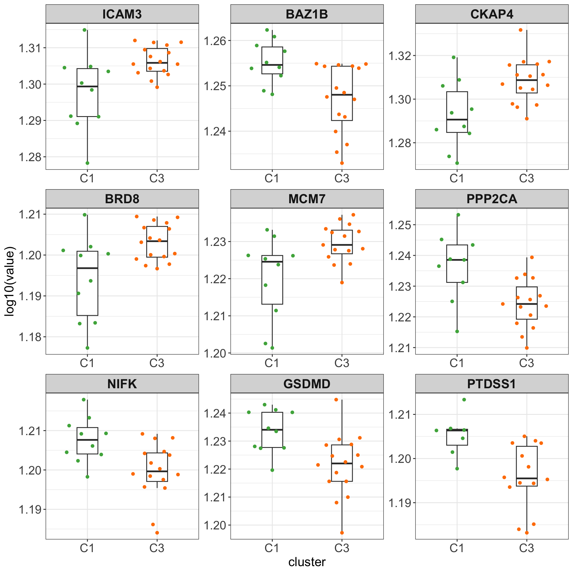
Association with BH3 profiling data
load("../../BH3profiling/output/dynamicBH3.RData")
dataBH3 <- dynamicBH3 %>% filter(drug == "DMSO", peptide != "DMSO") %>%
  distinct(patID, peptide, .keep_all = TRUE) %>%
  mutate(feature = peptide, value = AUC, concIndex =1) %>%
  mutate(cluster = clusterAnno[match(patID, clusterAnno$patientID),]$cluster) %>%
  filter(!is.na(cluster))

tRes <- group_by(dataBH3, feature) %>% nest() %>%
  mutate(m = map(data, ~t.test(value ~ cluster,., var.equal=TRUE))) %>%
  mutate(res = map(m, broom::tidy)) %>%
  unnest(res) %>%
  arrange(p.value)

head(tRes)
# A tibble: 6 × 13
# Groups: feature [6]
feature data m estimate estimate1 estimate2 statis…¹ p.value param…²
<chr> <list> <list> <dbl> <dbl> <dbl> <dbl> <dbl> <dbl>
1 BIM <tibble> <htest> -13.5 47.4 60.9 -2.08 0.0511 19
2 PUMA <tibble> <htest> -16.1 44.8 60.9 -2.07 0.0527 19
3 BAD <tibble> <htest> -12.3 61.1 73.5 -1.82 0.0840 19
4 FS1 <tibble> <htest> -10.5 18.0 28.5 -1.80 0.0881 19
5 HRKy <tibble> <htest> -3.80 -0.126 3.67 -1.61 0.123 19
6 MS1 <tibble> <htest> -12.9 29.5 42.4 -1.46 0.159 19
# … with 4 more variables: conf.low <dbl>, conf.high <dbl>, method <chr>,
# alternative <chr>, and abbreviated variable names ¹statistic, ²parameter
# ℹ Use `colnames()` to see all variable namesplotTab <- dataBH3 %>% filter(feature %in% c("FS1","MS1", "BIM"))
ggplot(plotTab, aes(x=cluster ,y = value)) +
geom_boxplot(width=0.5) +
geom_point(aes(col = cluster)) +
scale_color_manual(values = annoCol$cluster) +
facet_wrap(~feature) +
ylab("mitochondrial priming") + xlab("") +
theme_my + theme(legend.position = "none")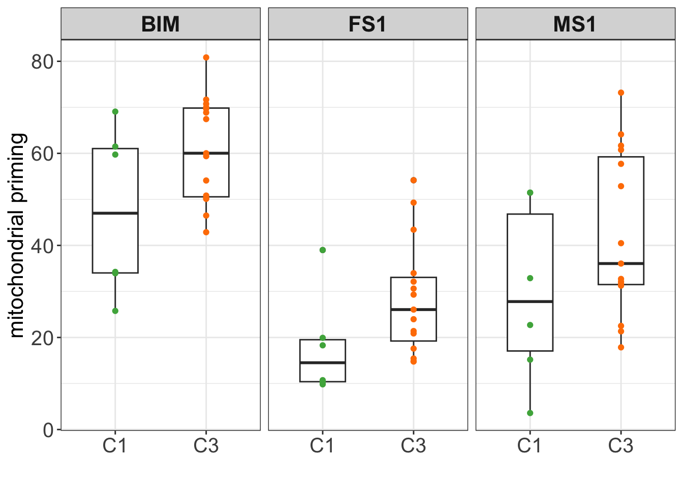
Association with treatment history
Only samples with BR therapy are enough for the test
load("../../var/inVivoEffect.RData")
testTab <- inVivoEffect %>% pivot_longer(-c(patientID, item)) %>%
  left_join(clusterTab, by = "patientID") %>%
  filter(cluster %in% c("C1","C3"), item == "BR", IGHV.status == "M")

table(testTab$name, testTab$cluster)
           C1 C3
  dropRate  2  3
  lymDrop   2  3
testRes <- group_by(testTab, name) %>% nest() %>%
mutate(m=map(data, ~t.test(value~cluster, ., var.equal = FALSE))) %>%
mutate(res = map(m, broom::tidy)) %>%
unnest(res)
testRes# A tibble: 2 × 13
# Groups: name [2]
name data m estimate estimate1 estimate2 stati…¹ p.value param…²
<chr> <list> <list> <dbl> <dbl> <dbl> <dbl> <dbl> <dbl>
1 lymDrop <tibble> <htest> -0.354 1.37 1.72 -1.01 0.418 2.04
2 dropRate <tibble> <htest> -0.00180 0.00649 0.00829 -1.60 0.225 2.48
# … with 4 more variables: conf.low <dbl>, conf.high <dbl>, method <chr>,
# alternative <chr>, and abbreviated variable names ¹statistic, ²parameter
# ℹ Use `colnames()` to see all variable namesggplot(testTab, aes(x=cluster, y = value, col = cluster)) +
#geom_boxplot(outlier.shape = NA, width =0.3) +
geom_point(size=3) +
scale_color_manual(values = annoCol$cluster) +
facet_wrap(~name, scale = "free") +
theme_my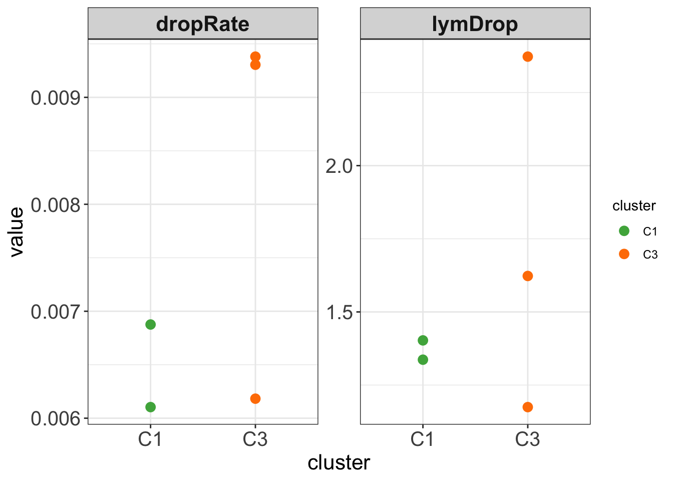
Compare the consistency of clustering in the three datasets (EMBL2016, CPS1000)
All patients
All samples
library(ggsankey)
cEMBL <- read_csv2("../output/consClust_EMBL2016.csv") %>%
  select(patientID, cluster) %>% dplyr::rename(EMBL2016 = cluster)
cCPS <- read_csv2("../output/consClust_CPS.csv") %>%
  select(patientID, cluster) %>% dplyr::rename(CPS1000 = cluster)
#cIC50 <- read_csv2("../output/consClust_IC50.csv") %>%
#  select(patientID, cluster) %>% dplyr::rename(IC50 = cluster)
comTab <- full_join(cEMBL, cCPS, by = "patientID") %>%
  #full_join(cIC50, by = "patientID") %>%
  filter(!is.na(EMBL2016),!is.na(CPS1000)) %>%
  make_long(EMBL2016, CPS1000)

ggplot(comTab, aes(x = x,
               next_x = next_x,
               node = node,
               next_node = next_node,
               fill = node)) +
  geom_sankey() +
  theme_sankey(base_size = 16) +
  xlab("")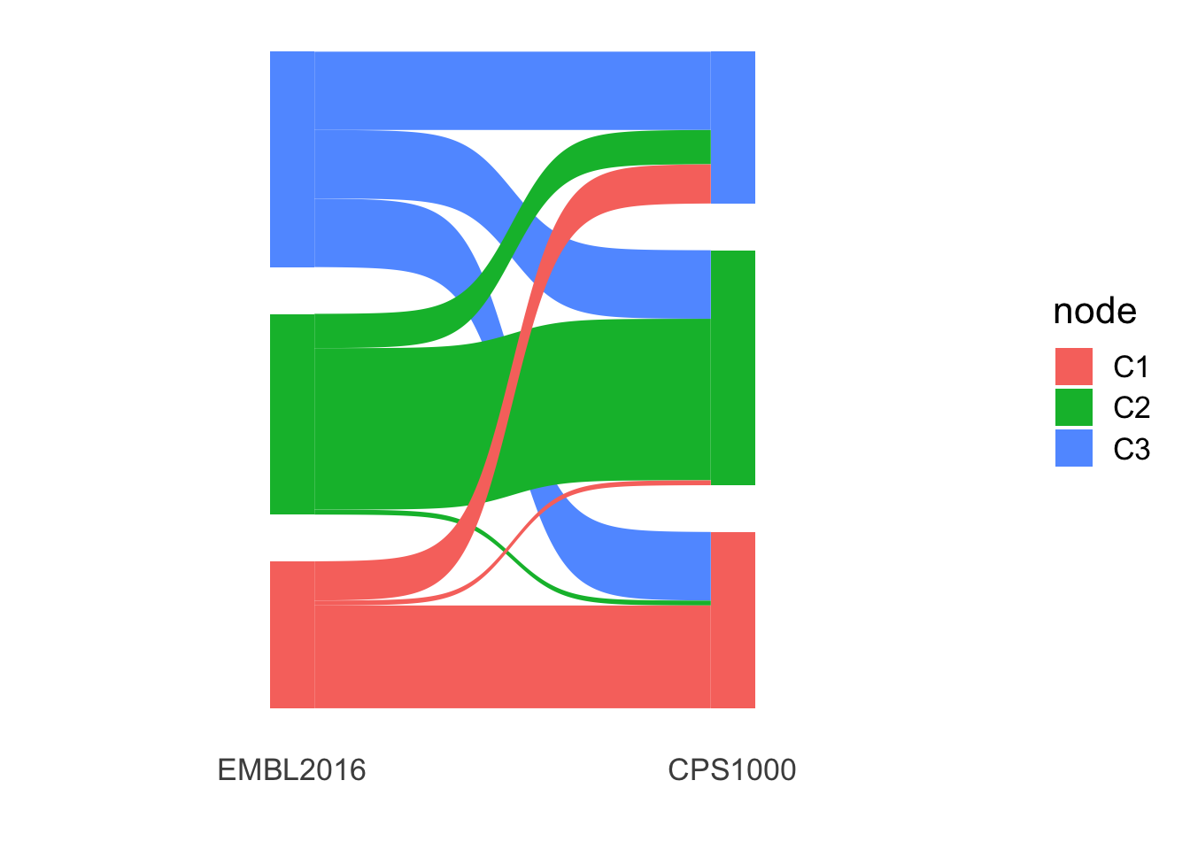
M-CLL samples
library(ggsankey)
cEMBL <- read_csv2("../output/consClust_EMBL2016.csv") %>%
filter(IGHV.status == "M") %>%
select(patientID, cluster) %>% dplyr::rename(EMBL2016 = cluster)
cCPS <- read_csv2("../output/consClust_CPS.csv") %>%
select(patientID, cluster) %>% dplyr::rename(CPS1000 = cluster)
#cIC50 <- read_csv2("../output/consClust_IC50.csv") %>%
# select(patientID, cluster) %>% dplyr::rename(IC50 = cluster)
comTab <- full_join(cEMBL, cCPS, by = "patientID") %>%
#full_join(cIC50, by = "patientID") %>%
filter(!is.na(EMBL2016),!is.na(CPS1000)) %>%
make_long(EMBL2016, CPS1000)
ggplot(comTab, aes(x = x,
next_x = next_x,
node = node,
next_node = next_node,
fill = node)) +
geom_sankey() +
theme_sankey(base_size = 16) +
xlab("")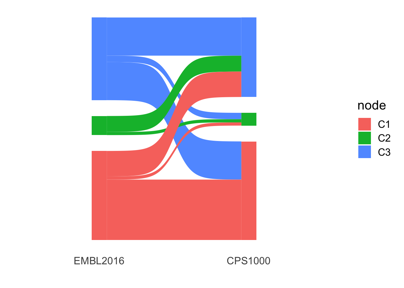 U-CLL samples
library(ggsankey)
cEMBL <- read_csv2("../output/consClust_EMBL2016.csv") %>%
  filter(IGHV.status == "U") %>%
  select(patientID, cluster) %>% dplyr::rename(EMBL2016 = cluster)
cCPS <- read_csv2("../output/consClust_CPS.csv") %>%
  select(patientID, cluster) %>% dplyr::rename(CPS1000 = cluster)
#cIC50 <- read_csv2("../output/consClust_IC50.csv") %>%
#  select(patientID, cluster) %>% dplyr::rename(IC50 = cluster)
comTab <- full_join(cEMBL, cCPS, by = "patientID") %>%
  #full_join(cIC50, by = "patientID") %>%
  filter(!is.na(EMBL2016),!is.na(CPS1000)) %>%
  make_long(EMBL2016, CPS1000)

ggplot(comTab, aes(x = x,
               next_x = next_x,
               node = node,
               next_node = next_node,
               fill = node)) +
  geom_sankey() +
  theme_sankey(base_size = 16) +
  xlab("")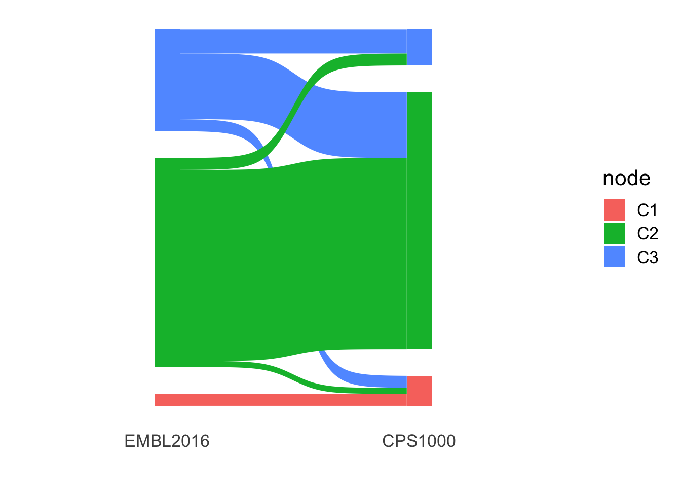
Only patients with the same samples used for both screens
Get the patient list with same samples used for both screens
load("~/CLLproject_jlu/var/CPS1000_mainAnalysis.RData")
cpsScreen <- pheno1000_main
load("../output/screenData.RData")
emblScreen <- screenData
overSample <- intersect(cpsScreen$sampleID, emblScreen$sampleID)
overPat <- filter(emblScreen, sampleID %in% overSample)$patientID
Compare all CLL samples
All samples
library(ggsankey)
cEMBL <- read_csv2("../output/consClust_EMBL2016.csv") %>%
  select(patientID, cluster) %>% dplyr::rename(EMBL2016 = cluster)
cCPS <- read_csv2("../output/consClust_CPS.csv") %>%
  select(patientID, cluster) %>% dplyr::rename(CPS1000 = cluster)
#cIC50 <- read_csv2("../output/consClust_IC50.csv") %>%
#  select(patientID, cluster) %>% dplyr::rename(IC50 = cluster)
comTab <- full_join(cEMBL, cCPS, by = "patientID") %>%
  filter(patientID %in% overPat) %>%
  #full_join(cIC50, by = "patientID") %>%
  filter(!is.na(EMBL2016),!is.na(CPS1000)) %>%
  make_long(EMBL2016, CPS1000)

ggplot(comTab, aes(x = x,
               next_x = next_x,
               node = node,
               next_node = next_node,
               fill = node)) +
  geom_sankey() +
  theme_sankey(base_size = 16) +
  xlab("")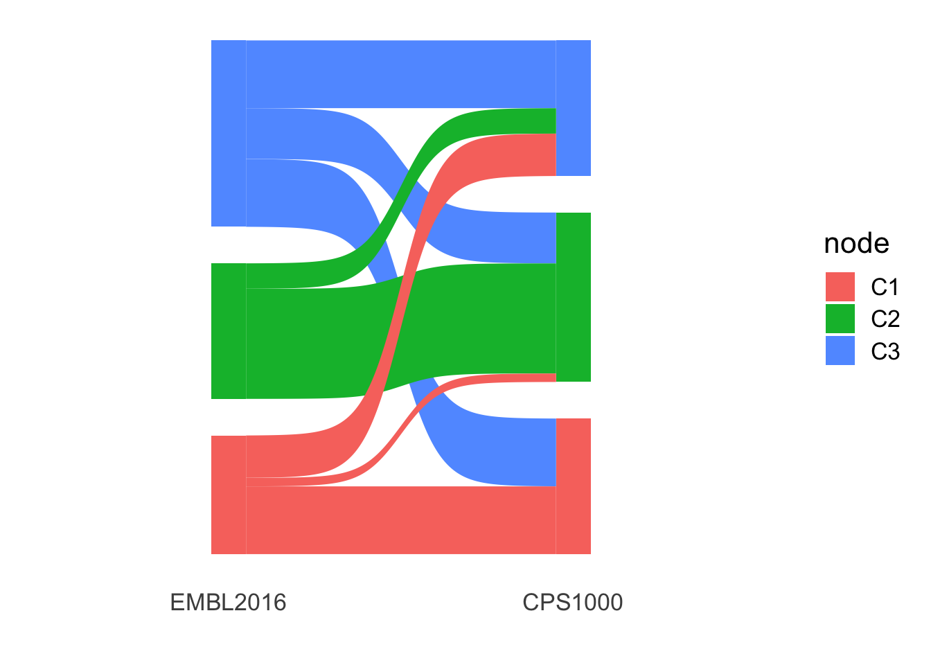
M-CLL samples
library(ggsankey)
cEMBL <- read_csv2("../output/consClust_EMBL2016.csv") %>%
filter(IGHV.status == "M") %>%
select(patientID, cluster) %>% dplyr::rename(EMBL2016 = cluster)
cCPS <- read_csv2("../output/consClust_CPS.csv") %>%
select(patientID, cluster) %>% dplyr::rename(CPS1000 = cluster)
#cIC50 <- read_csv2("../output/consClust_IC50.csv") %>%
# select(patientID, cluster) %>% dplyr::rename(IC50 = cluster)
comTab <- full_join(cEMBL, cCPS, by = "patientID") %>%
filter(patientID %in% overPat) %>%
#full_join(cIC50, by = "patientID") %>%
filter(!is.na(EMBL2016),!is.na(CPS1000)) %>%
make_long(EMBL2016, CPS1000)
ggplot(comTab, aes(x = x,
next_x = next_x,
node = node,
next_node = next_node,
fill = node)) +
geom_sankey() +
theme_sankey(base_size = 16) +
xlab("")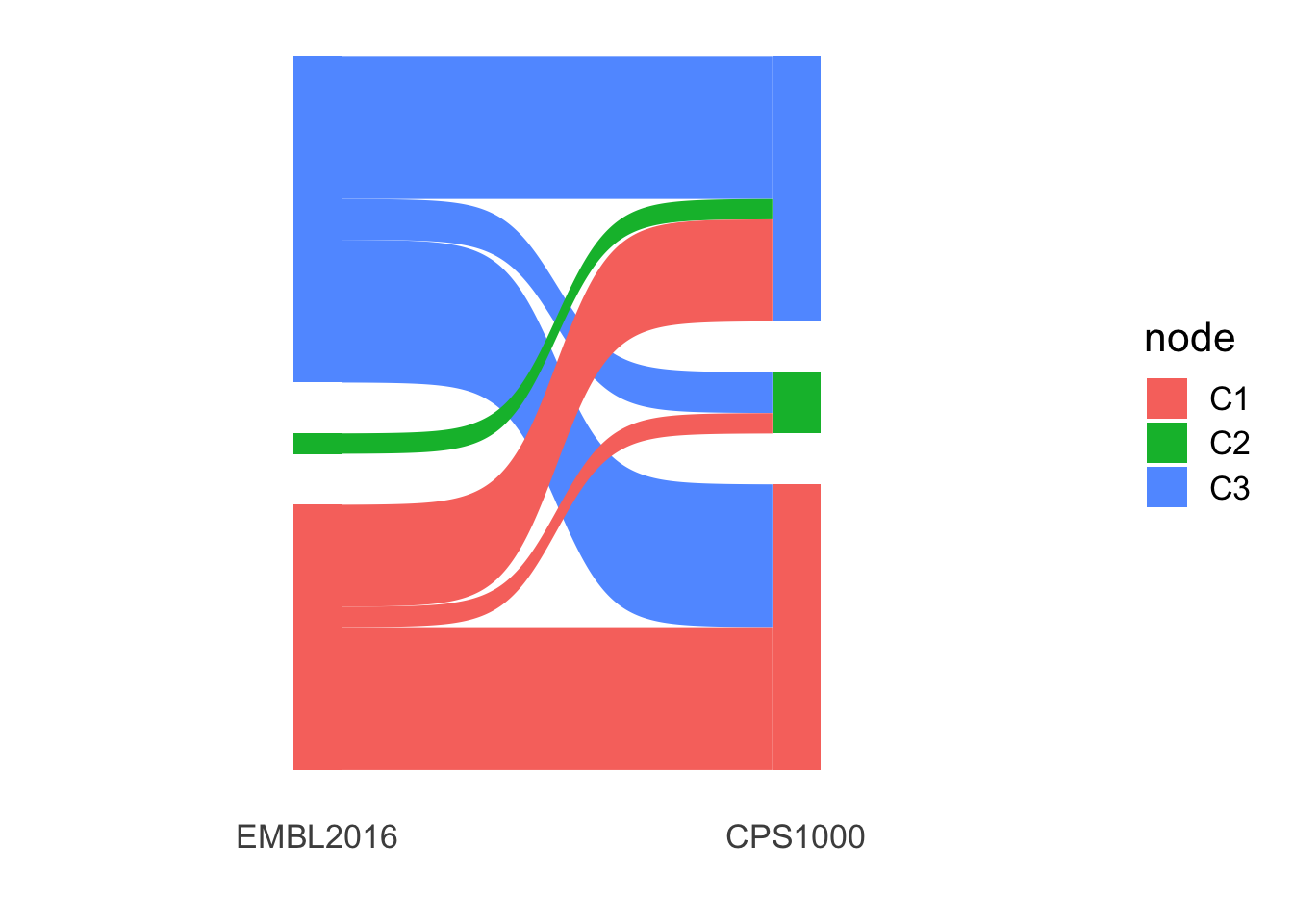 U-CLL samples
library(ggsankey)
cEMBL <- read_csv2("../output/consClust_EMBL2016.csv") %>%
  filter(IGHV.status == "U") %>%
  select(patientID, cluster) %>% dplyr::rename(EMBL2016 = cluster)
cCPS <- read_csv2("../output/consClust_CPS.csv") %>%
  select(patientID, cluster) %>% dplyr::rename(CPS1000 = cluster)
#cIC50 <- read_csv2("../output/consClust_IC50.csv") %>%
#  select(patientID, cluster) %>% dplyr::rename(IC50 = cluster)
comTab <- full_join(cEMBL, cCPS, by = "patientID") %>%
  filter(patientID %in% overPat) %>%
  #full_join(cIC50, by = "patientID") %>%
  filter(!is.na(EMBL2016),!is.na(CPS1000)) %>%
  make_long(EMBL2016, CPS1000)

ggplot(comTab, aes(x = x,
               next_x = next_x,
               node = node,
               next_node = next_node,
               fill = node)) +
  geom_sankey() +
  theme_sankey(base_size = 16) +
  xlab("")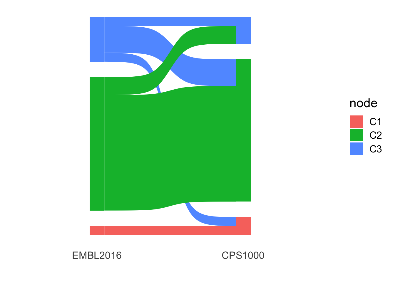
sessionInfo()R version 4.2.0 (2022-04-22)
Platform: x86_64-apple-darwin17.0 (64-bit)
Running under: macOS Big Sur/Monterey 10.16
Matrix products: default
BLAS: /Library/Frameworks/R.framework/Versions/4.2/Resources/lib/libRblas.0.dylib
LAPACK: /Library/Frameworks/R.framework/Versions/4.2/Resources/lib/libRlapack.dylib
locale:
[1] en_US.UTF-8/en_US.UTF-8/en_US.UTF-8/C/en_US.UTF-8/en_US.UTF-8
attached base packages:
[1] stats4 stats graphics grDevices utils datasets methods
[8] base
other attached packages:
[1] ggsankey_0.0.99999 forcats_0.5.1
[3] stringr_1.4.1 dplyr_1.0.9
[5] purrr_0.3.4 readr_2.1.2
[7] tidyr_1.2.0 tibble_3.1.8
[9] tidyverse_1.3.2 missForest_1.5
[11] Rtsne_0.16 pheatmap_1.0.12
[13] proDA_1.10.0 DESeq2_1.36.0
[15] SummarizedExperiment_1.26.1 Biobase_2.56.0
[17] MatrixGenerics_1.8.1 matrixStats_0.62.0
[19] GenomicRanges_1.48.0 GenomeInfoDb_1.32.2
[21] IRanges_2.30.0 S4Vectors_0.34.0
[23] BiocGenerics_0.42.0 survminer_0.4.9
[25] ggpubr_0.4.0 ggplot2_3.4.1
[27] survival_3.4-0 cowplot_1.1.1
[29] ConsensusClusterPlus_1.60.0
loaded via a namespace (and not attached):
[1] shinydashboard_0.7.2 utf8_1.2.2 tidyselect_1.1.2
[4] htmlwidgets_1.5.4 RSQLite_2.2.15 AnnotationDbi_1.58.0
[7] grid_4.2.0 BiocParallel_1.30.3 maxstat_0.7-25
[10] munsell_0.5.0 ragg_1.2.2 codetools_0.2-18
[13] DT_0.23 withr_2.5.0 colorspace_2.0-3
[16] highr_0.9 knitr_1.39 rstudioapi_0.13
[19] ggsignif_0.6.3 labeling_0.4.2 git2r_0.30.1
[22] slam_0.1-50 GenomeInfoDbData_1.2.8 KMsurv_0.1-5
[25] bit64_4.0.5 farver_2.1.1 rprojroot_2.0.3
[28] vctrs_0.5.2 generics_0.1.3 TH.data_1.1-1
[31] xfun_0.31 itertools_0.1-3 randomForest_4.7-1.1
[34] sets_1.0-21 markdown_1.1 R6_2.5.1
[37] ggbeeswarm_0.6.0 locfit_1.5-9.6 fgsea_1.22.0
[40] bitops_1.0-7 cachem_1.0.6 DelayedArray_0.22.0
[43] assertthat_0.2.1 promises_1.2.0.1 scales_1.2.0
[46] vroom_1.5.7 multcomp_1.4-19 googlesheets4_1.0.0
[49] beeswarm_0.4.0 gtable_0.3.0 extraDistr_1.9.1
[52] sandwich_3.0-2 workflowr_1.7.0 rlang_1.0.6
[55] genefilter_1.78.0 systemfonts_1.0.4 splines_4.2.0
[58] rstatix_0.7.0 gargle_1.2.0 broom_1.0.0
[61] BiocManager_1.30.18 yaml_2.3.5 abind_1.4-5
[64] modelr_0.1.8 crosstalk_1.2.0 backports_1.4.1
[67] httpuv_1.6.6 gridtext_0.1.4 tools_4.2.0
[70] relations_0.6-12 ellipsis_0.3.2 gplots_3.1.3
[73] jquerylib_0.1.4 RColorBrewer_1.1-3 Rcpp_1.0.9
[76] visNetwork_2.1.0 zlibbioc_1.42.0 RCurl_1.98-1.7
[79] zoo_1.8-10 ggrepel_0.9.1 haven_2.5.0
[82] cluster_2.1.3 exactRankTests_0.8-35 fs_1.5.2
[85] magrittr_2.0.3 data.table_1.14.2 reprex_2.0.1
[88] googledrive_2.0.0 mvtnorm_1.1-3 shinyjs_2.1.0
[91] hms_1.1.1 mime_0.12 evaluate_0.15
[94] xtable_1.8-4 XML_3.99-0.10 readxl_1.4.0
[97] gridExtra_2.3 compiler_4.2.0 KernSmooth_2.23-20
[100] crayon_1.5.2 htmltools_0.5.4 later_1.3.0
[103] tzdb_0.3.0 ggtext_0.1.1 geneplotter_1.74.0
[106] lubridate_1.8.0 DBI_1.1.3 dbplyr_2.2.1
[109] MASS_7.3-58 jyluMisc_0.1.5 BiocStyle_2.24.0
[112] Matrix_1.4-1 car_3.1-0 cli_3.4.1
[115] marray_1.74.0 parallel_4.2.0 igraph_1.3.4
[118] pkgconfig_2.0.3 km.ci_0.5-6 piano_2.12.0
[121] xml2_1.3.3 foreach_1.5.2 annotate_1.74.0
[124] vipor_0.4.5 bslib_0.4.1 rngtools_1.5.2
[127] XVector_0.36.0 drc_3.0-1 rvest_1.0.2
[130] doRNG_1.8.2 digest_0.6.30 Biostrings_2.64.0
[133] fastmatch_1.1-3 rmarkdown_2.14 cellranger_1.1.0
[136] survMisc_0.5.6 shiny_1.7.4 gtools_3.9.3
[139] lifecycle_1.0.3 jsonlite_1.8.3 carData_3.0-5
[142] limma_3.52.2 fansi_1.0.3 pillar_1.8.0
[145] lattice_0.20-45 KEGGREST_1.36.3 fastmap_1.1.0
[148] httr_1.4.3 plotrix_3.8-2 glue_1.6.2
[151] png_0.1-7 iterators_1.0.14 bit_4.0.4
[154] stringi_1.7.8 sass_0.4.2 blob_1.2.3
[157] textshaping_0.3.6 caTools_1.18.2 memoise_2.0.1