Identify disease specific drug responses
Junyan Lu
6 May 2022
Last updated: 2022-05-06
Checks: 6 1
Knit directory: EMBL2016/analysis/
This reproducible R Markdown analysis was created with workflowr (version 1.7.0). The Checks tab describes the reproducibility checks that were applied when the results were created. The Past versions tab lists the development history.
The R Markdown is untracked by Git. To know which version of the R Markdown file created these results, you’ll want to first commit it to the Git repo. If you’re still working on the analysis, you can ignore this warning. When you’re finished, you can run wflow_publish to commit the R Markdown file and build the HTML.
Great job! The global environment was empty. Objects defined in the global environment can affect the analysis in your R Markdown file in unknown ways. For reproduciblity it’s best to always run the code in an empty environment.
The command set.seed(20210512) was run prior to running the code in the R Markdown file. Setting a seed ensures that any results that rely on randomness, e.g. subsampling or permutations, are reproducible.
Great job! Recording the operating system, R version, and package versions is critical for reproducibility.
Nice! There were no cached chunks for this analysis, so you can be confident that you successfully produced the results during this run.
Great job! Using relative paths to the files within your workflowr project makes it easier to run your code on other machines.
Great! You are using Git for version control. Tracking code development and connecting the code version to the results is critical for reproducibility.
The results in this page were generated with repository version 12d1722. See the Past versions tab to see a history of the changes made to the R Markdown and HTML files.
Note that you need to be careful to ensure that all relevant files for the analysis have been committed to Git prior to generating the results (you can use wflow_publish or wflow_git_commit). workflowr only checks the R Markdown file, but you know if there are other scripts or data files that it depends on. Below is the status of the Git repository when the results were generated:
Ignored files:
    Ignored:    .DS_Store
    Ignored:    .Rhistory
    Ignored:    analysis/.DS_Store
    Ignored:    analysis/.Rhistory
    Ignored:    analysis/boxplot_AUC.png
    Ignored:    analysis/consensus_clustering_CPS_cache/
    Ignored:    analysis/consensus_clustering_noFit_cache/
    Ignored:    analysis/dose_curve.png
    Ignored:    analysis/targetDist.png
    Ignored:    analysis/toxivity_box.png
    Ignored:    analysis/volcano.png
    Ignored:    data/.DS_Store
    Ignored:    output/.DS_Store

Untracked files:
    Untracked:  analysis/AUC_CLL_IC50/
    Untracked:  analysis/BRAF_analysis.Rmd
    Untracked:  analysis/GSVA_analysis.Rmd
    Untracked:  analysis/NOTCH1_signature.Rmd
    Untracked:  analysis/autoluminescence.Rmd
    Untracked:  analysis/bar_plot_mixed.pdf
    Untracked:  analysis/bar_plot_mixed_noU1.pdf
    Untracked:  analysis/beatAML/
    Untracked:  analysis/cohortComposition_CLLsamples.pdf
    Untracked:  analysis/cohortComposition_allSamples.pdf
    Untracked:  analysis/consensus_clustering.Rmd
    Untracked:  analysis/consensus_clustering_CPS.Rmd
    Untracked:  analysis/consensus_clustering_IC50.Rmd
    Untracked:  analysis/consensus_clustering_beatAML.Rmd
    Untracked:  analysis/consensus_clustering_noFit.Rmd
    Untracked:  analysis/consensus_clusters.pdf
    Untracked:  analysis/disease_specific.Rmd
    Untracked:  analysis/dose_curve_selected.pdf
    Untracked:  analysis/genomic_association.Rmd
    Untracked:  analysis/genomic_association_allDisease.Rmd
    Untracked:  analysis/mean_autoluminescence_val.csv
    Untracked:  analysis/mean_autoluminescence_val.xlsx
    Untracked:  analysis/noFit_CLL/
    Untracked:  analysis/number_associations.pdf
    Untracked:  analysis/overview.Rmd
    Untracked:  analysis/plotCohort.Rmd
    Untracked:  analysis/preprocess.Rmd
    Untracked:  analysis/volcano_noBlocking.pdf
    Untracked:  code/utils.R
    Untracked:  data/BeatAML_Waves1_2/
    Untracked:  data/ic50Tab.RData
    Untracked:  data/newEMBL_20210806.RData
    Untracked:  data/patMeta.RData
    Untracked:  data/targetAnnotation_all.csv
    Untracked:  force_sync.sh
    Untracked:  output/gene_associations/
    Untracked:  output/resConsClust.RData
    Untracked:  output/resConsClust_aucFit.RData
    Untracked:  output/resConsClust_beatAML.RData
    Untracked:  output/resConsClust_cps.RData
    Untracked:  output/resConsClust_ic50.RData
    Untracked:  output/resConsClust_noFit.RData
    Untracked:  output/screenData.RData
    Untracked:  sync.sh

Unstaged changes:
    Modified:   _workflowr.yml
    Modified:   analysis/_site.yml
    Deleted:    analysis/about.Rmd
    Modified:   analysis/index.Rmd
    Deleted:    analysis/license.Rmd
Note that any generated files, e.g. HTML, png, CSS, etc., are not included in this status report because it is ok for generated content to have uncommitted changes.
There are no past versions. Publish this analysis with wflow_publish() to start tracking its development.
Load libraries and dataset
Load datasets
Disease stratification by drug response phenotypes
T-sne plot
Get disease types with at least 3 cases
diagTab <- screenData %>% distinct(patientID, diagnosis) %>%
  group_by(diagnosis) %>% summarise(n=length(patientID)) %>%
  arrange(n)
filter(diagTab, n>=3)
# A tibble: 6 × 2
diagnosis n
<chr> <int>
1 B-NHL 3
2 B-PLL 3
3 T-PLL 8
4 MCL 10
5 AML 14
6 CLL 132
UMAP (alternative for T-SNE)
#Calculate UMAP layout, which can better retain global structure
plotTab <- smallvis(t(viabMat), method = "umap", perplexity = 30,
                    eta = 0.01, epoch_callback = FALSE, verbose = FALSE)
colnames(plotTab) <- c("x","y")

plotTab <- plotTab %>% as.tibble() %>% mutate(Patient.ID = colnames(viabMat)) %>%
  left_join(select(patMeta, Patient.ID, diagnosis, IGHV.status, project), by = "Patient.ID") %>%
  mutate(diagnosis = as.character(diagnosis), project = as.character(project)) %>%
  mutate(diagnosis = ifelse(diagnosis == "CLL" & IGHV.status == "U", "U-CLL",diagnosis)) %>%
  filter(!is.na(diagnosis))
UMAP plot (better retain global structure) 
Hierarchical clustering & heatmap
All samples
NA values will cause problem of hierarchical clustering
Evaluate the completeness of data points
plotTab <- filter(screenData, ! Drug %in% c("DMSO","PBS")) %>%
  #filter(diagnosis %in% c("CLL","MCL","T-PLL","MZL","B-NHL","B-PLL","Sezary")) %>% #only disease with more than 2 cases
  group_by(patientID, Drug) %>% summarise(viab = mean(viab.auc, na.rm=TRUE)) %>% ungroup()

sumTab <- group_by(plotTab, Drug) %>% summarise(noNA = sum(!is.na(viab)), fracNoNA = sum(!is.na(viab))/length(patientID)) %>%
  arrange(desc(fracNoNA)) %>% ungroup() %>% mutate(Drug = factor(Drug, levels = Drug))

ggplot(sumTab, aes(x=Drug, y = fracNoNA)) + geom_point() +
  ylab("Fraction of successfully fitted values") +
  theme(axis.text.x = element_text(angle = 90, hjust=1, vjust=0.5))
In this part, only disease that have at least 2 cases will be included. There are 145 out of 166 samples passed the criteria.
Only include samples that have at least 50% non-missing vlaues
sumPatTab <- group_by(plotTab, patientID) %>%
  summarise(noNA = sum(!is.na(viab)), fracNoNA = sum(!is.na(viab))/length(patientID)) %>%
  arrange(desc(fracNoNA)) %>% ungroup()
usePat <- filter(sumPatTab, fracNoNA >= 0.5)$patientID
How many samples will be included?
length(usePat)[1] 186How many drugs will be included?
length(filter(sumTab, fracNoNA > 0.2)$Drug)[1] 408Prepare viability matrix
plotMat <- plotTab %>% filter(Drug %in% filter(sumTab, fracNoNA > 0.2)$Drug, patientID %in% usePat) %>%
  spread(key = patientID, value = "viab") %>% data.frame() %>%
  column_to_rownames("Drug") %>% as.matrix()

#Prepare data

#plotMat.complete <- plotMat[complete.cases(plotMat),]

#center by mean and scale by MAD
#plotMat <- jyluMisc::mscale(plotMat, censor = 4, useMad = TRUE)
Heatmap (row centered by median and scaled by MAD)  PDF version: heatmap_all-1.pdf
Only plot the tree for identifying clusters  PDF version: tree_all-1.pdf
Boxplot with the same order of rows in the heatmap above
dOrder <- p$tree_row$labels[p$tree_row$order]
plotTabBox <- plotMat %>% as_tibble(rownames = "Drug") %>%
  pivot_longer(-Drug, names_to = "patID", values_to = "auc") %>%
  mutate(Drug = factor(Drug, levels = dOrder))

ggplot(plotTabBox, aes(x=Drug, y=auc)) +
  geom_boxplot() +
  coord_flip() +
  theme_bw() +
  theme(axis.text.y = element_blank(),
        axis.ticks.y = element_blank(),
        panel.grid = element_blank()) +
  xlab("") +
  ylab("AUC")
PDF version: sideBox_all-1.pdf
Only CLL
Evaluate the completeness of data points
plotTab <- filter(screenData, ! Drug %in% c("DMSO","PBS")) %>%
filter(diagnosis %in% c("CLL")) %>%
group_by(patientID, Drug) %>% summarise(viab = mean(viab.auc, na.rm=TRUE)) %>% ungroup()
sumTab <- group_by(plotTab, Drug) %>% summarise(noNA = sum(!is.na(viab)), fracNoNA = sum(!is.na(viab))/length(patientID)) %>%
arrange(desc(fracNoNA)) %>% ungroup() %>% mutate(Drug = factor(Drug, levels = Drug))
ggplot(sumTab, aes(x=Drug, y = fracNoNA)) + geom_point() +
ylab("Fraction of successfully fitted values") +
theme(axis.text.x = element_text(angle = 90, hjust=1, vjust=0.5))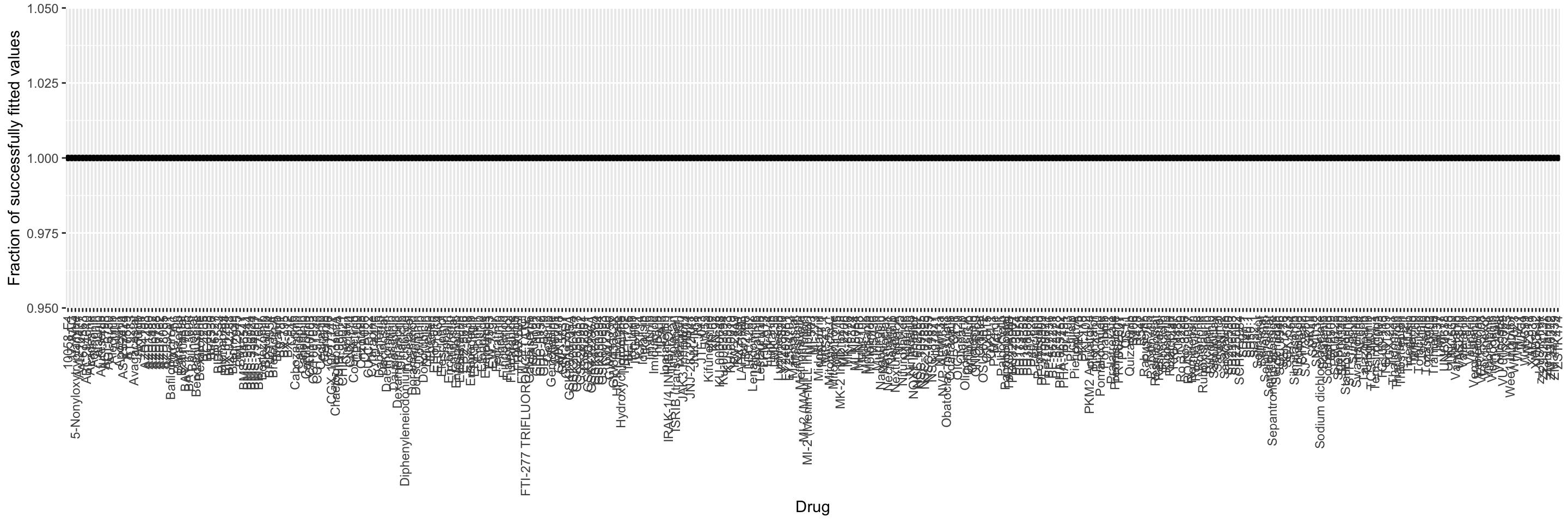 How many drugs will be included?
length(filter(sumTab, fracNoNA > 0.2)$Drug)[1] 408Prepare viability matrix
plotMat <- plotTab %>% filter(Drug %in% filter(sumTab, fracNoNA > 0.2)$Drug) %>%
  spread(key = patientID, value = "viab") %>% data.frame() %>%
  column_to_rownames("Drug") %>% as.matrix()

#Prepare data

#plotMat.complete <- plotMat[complete.cases(plotMat),]

#center by mean and scale by MAD
#plotMat <- jyluMisc::mscale(plotMat, censor = 4, useMad = TRUE)
Heatmap plot (row centered by median and scaled by MAD) 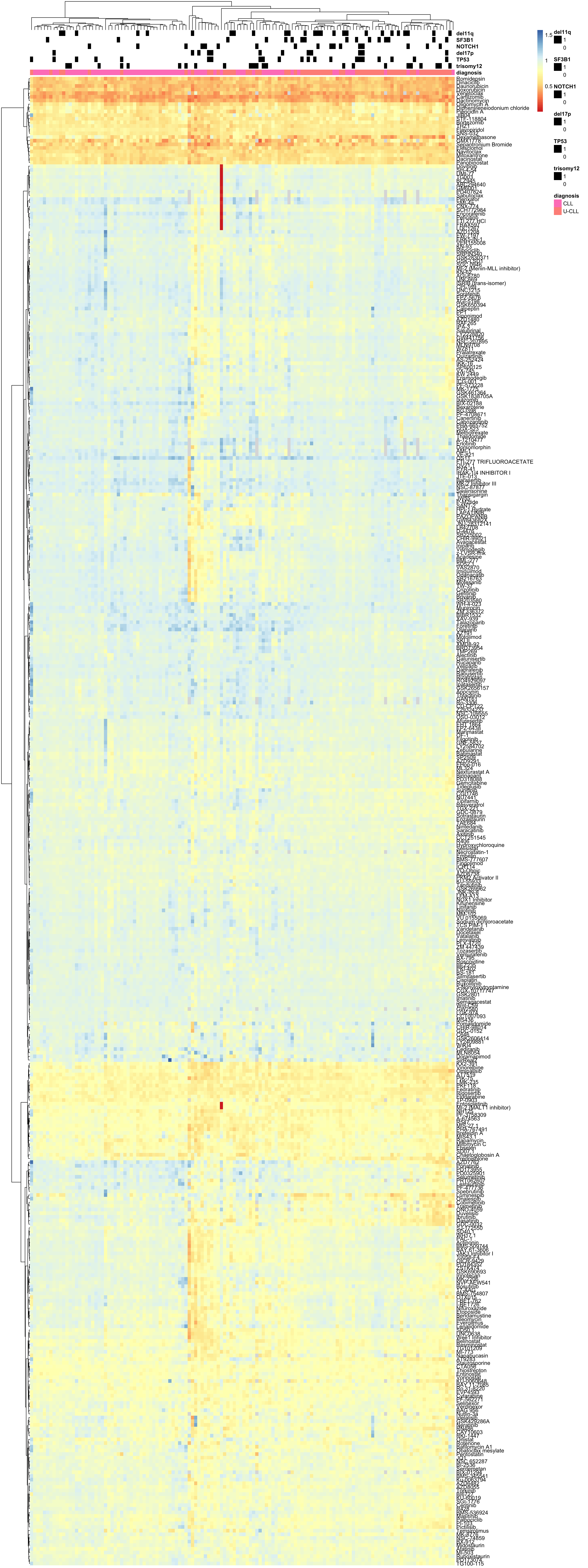 PDF version: heatmap_CLL-1.pdf
Only plot the tree for identifying clusters  PDF version: tree_CLL-1.pdf
Boxplot with the same order of rows in the heatmap above
dOrder <- p$tree_row$labels[p$tree_row$order]
plotTabBox <- plotMat %>% as_tibble(rownames = "Drug") %>%
  pivot_longer(-Drug, names_to = "patID", values_to = "auc") %>%
  mutate(Drug = factor(Drug, levels = dOrder))

ggplot(plotTabBox, aes(x=Drug, y=auc)) +
  geom_boxplot() +
  coord_flip() +
  theme_bw() +
  theme(axis.text.y = element_blank(),
        axis.ticks.y = element_blank(),
        panel.grid = element_blank()) +
  xlab("") +
  ylab("AUC")
PDF version: sideBox_cll-1.pdf
Disease-specific drug effect
[1] "AML"
[1] "MCL"
[1] "T-PLL"
[1] "B-NHL"
[1] "B-PLL"
p value heatmap 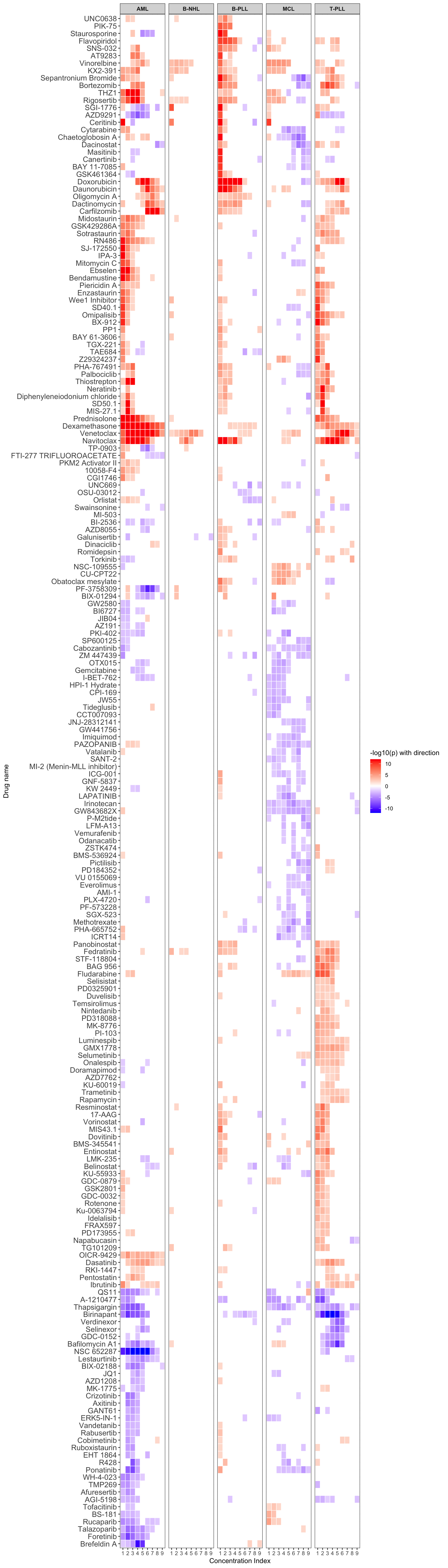 PDF version
Blue means increased sensitivity compared to CLL, while red means increased resistance. (only drugs that have associations in at least 3 concentrations are shown, FDR = 10%)
sessionInfo()R version 4.1.2 (2021-11-01)
Platform: x86_64-apple-darwin17.0 (64-bit)
Running under: macOS Big Sur 10.16
Matrix products: default
BLAS: /Library/Frameworks/R.framework/Versions/4.1/Resources/lib/libRblas.0.dylib
LAPACK: /Library/Frameworks/R.framework/Versions/4.1/Resources/lib/libRlapack.dylib
locale:
[1] en_US.UTF-8/en_US.UTF-8/en_US.UTF-8/C/en_US.UTF-8/en_US.UTF-8
attached base packages:
[1] stats graphics grDevices utils datasets methods base
other attached packages:
[1] forcats_0.5.1 stringr_1.4.0 dplyr_1.0.7
[4] purrr_0.3.4 readr_2.1.1 tidyr_1.1.4
[7] tibble_3.1.6 tidyverse_1.3.1 limma_3.50.0
[10] readxl_1.3.1 gtable_0.3.0 glmnet_4.1-3
[13] Matrix_1.4-0 ggbeeswarm_0.6.0 jyluMisc_0.1.5
[16] colorspace_2.0-2 RColorBrewer_1.1-2 ggrepel_0.9.1
[19] ggplot2_3.3.5 smallvis_0.0.0.9000 Rtsne_0.15
[22] cowplot_1.1.1 genefilter_1.76.0 pheatmap_1.0.12
[25] reshape2_1.4.4 gridExtra_2.3 Biobase_2.54.0
[28] BiocGenerics_0.40.0
loaded via a namespace (and not attached):
[1] utf8_1.2.2 shinydashboard_0.7.2
[3] tidyselect_1.1.1 RSQLite_2.2.9
[5] AnnotationDbi_1.56.2 htmlwidgets_1.5.4
[7] grid_4.1.2 BiocParallel_1.28.3
[9] maxstat_0.7-25 munsell_0.5.0
[11] codetools_0.2-18 DT_0.20
[13] withr_2.4.3 highr_0.9
[15] knitr_1.37 rstudioapi_0.13
[17] stats4_4.1.2 ggsignif_0.6.3
[19] MatrixGenerics_1.6.0 labeling_0.4.2
[21] git2r_0.29.0 slam_0.1-50
[23] GenomeInfoDbData_1.2.7 KMsurv_0.1-5
[25] farver_2.1.0 bit64_4.0.5
[27] rprojroot_2.0.2 vctrs_0.3.8
[29] generics_0.1.1 TH.data_1.1-0
[31] xfun_0.29 sets_1.0-20
[33] R6_2.5.1 GenomeInfoDb_1.30.0
[35] bitops_1.0-7 cachem_1.0.6
[37] fgsea_1.20.0 DelayedArray_0.20.0
[39] assertthat_0.2.1 promises_1.2.0.1
[41] scales_1.1.1 multcomp_1.4-18
[43] beeswarm_0.4.0 sandwich_3.0-1
[45] workflowr_1.7.0 rlang_0.4.12
[47] splines_4.1.2 rstatix_0.7.0
[49] broom_0.7.11 BiocManager_1.30.16
[51] yaml_2.2.1 abind_1.4-5
[53] modelr_0.1.8 backports_1.4.1
[55] httpuv_1.6.5 tools_4.1.2
[57] relations_0.6-10 ellipsis_0.3.2
[59] gplots_3.1.1 jquerylib_0.1.4
[61] Rcpp_1.0.8 plyr_1.8.6
[63] visNetwork_2.1.0 zlibbioc_1.40.0
[65] RCurl_1.98-1.5 ggpubr_0.4.0
[67] S4Vectors_0.32.3 zoo_1.8-9
[69] SummarizedExperiment_1.24.0 haven_2.4.3
[71] cluster_2.1.2 exactRankTests_0.8-34
[73] fs_1.5.2 magrittr_2.0.1
[75] data.table_1.14.2 reprex_2.0.1
[77] survminer_0.4.9 mvtnorm_1.1-3
[79] matrixStats_0.61.0 hms_1.1.1
[81] shinyjs_2.1.0 mime_0.12
[83] evaluate_0.14 xtable_1.8-4
[85] XML_3.99-0.8 IRanges_2.28.0
[87] shape_1.4.6 compiler_4.1.2
[89] KernSmooth_2.23-20 crayon_1.4.2
[91] htmltools_0.5.2 later_1.3.0
[93] tzdb_0.2.0 lubridate_1.8.0
[95] DBI_1.1.2 dbplyr_2.1.1
[97] MASS_7.3-55 BiocStyle_2.22.0
[99] car_3.0-12 cli_3.1.1
[101] marray_1.72.0 parallel_4.1.2
[103] igraph_1.2.11 GenomicRanges_1.46.1
[105] pkgconfig_2.0.3 km.ci_0.5-2
[107] piano_2.10.0 xml2_1.3.3
[109] foreach_1.5.1 annotate_1.72.0
[111] vipor_0.4.5 bslib_0.3.1
[113] XVector_0.34.0 drc_3.0-1
[115] rvest_1.0.2 digest_0.6.29
[117] Biostrings_2.62.0 rmarkdown_2.11
[119] cellranger_1.1.0 fastmatch_1.1-3
[121] survMisc_0.5.5 shiny_1.7.1
[123] gtools_3.9.2 lifecycle_1.0.1
[125] jsonlite_1.7.3 carData_3.0-5
[127] fansi_1.0.2 pillar_1.6.5
[129] lattice_0.20-45 KEGGREST_1.34.0
[131] fastmap_1.1.0 httr_1.4.2
[133] plotrix_3.8-2 survival_3.2-13
[135] glue_1.6.1 FNN_1.1.3
[137] png_0.1-7 iterators_1.0.13
[139] bit_4.0.4 stringi_1.7.6
[141] sass_0.4.0 blob_1.2.2
[143] caTools_1.18.2 memoise_2.0.1