Identify proteins associated with random node group of baseline samples (Visit 3)
Junyan Lu
17 May 2024
Last updated: 2024-05-17
Checks: 5 1
Knit directory:
SpinalCord_proteomics/analysis/
This reproducible R Markdown analysis was created with workflowr (version 1.7.0). The Checks tab describes the reproducibility checks that were applied when the results were created. The Past versions tab lists the development history.
Great job! The global environment was empty. Objects defined in the global environment can affect the analysis in your R Markdown file in unknown ways. For reproduciblity it’s best to always run the code in an empty environment.
The command set.seed(20221110) was run prior to running
the code in the R Markdown file. Setting a seed ensures that any results
that rely on randomness, e.g. subsampling or permutations, are
reproducible.
Great job! Recording the operating system, R version, and package versions is critical for reproducibility.
Nice! There were no cached chunks for this analysis, so you can be confident that you successfully produced the results during this run.
Great job! Using relative paths to the files within your workflowr project makes it easier to run your code on other machines.
Tracking code development and connecting the code version to the
results is critical for reproducibility. To start using Git, open the
Terminal and type git init in your project directory.
This project is not being versioned with Git. To obtain the full
reproducibility benefits of using workflowr, please see
?wflow_start.
Look at the structure of baseline patient samples with injury
Preprocessing the data with only injury samples
seProt_corr <- prepareProt(seProt, filterCondi = list(Treatment = c("0","1")), perNA = 1)[1] "Number of proteins: 473, number of samples: 318"patAnno <- colData(seProt_corr)
patAnno$Visit <- factor(ifelse(is.na(patAnno$Visit),0, patAnno$Visit))
patAnno$delta_UEMS <- ifelse(is.na(patAnno$delta_UEMS),0, patAnno$delta_UEMS)
patAnno$UEMS <- ifelse(is.na(patAnno$UEMS),0, patAnno$UEMS)
patAnno$AIS <- ifelse(is.na(patAnno$AIS),"None", patAnno$AIS)
patAnno$treatVis <- paste0(patAnno$Treatment, patAnno$Visit)
patAnno$nodeGroup <- factor(patAnno$nodeGroup)
mod <- model.matrix(~ Treatment + Visit + nodeGroup + UEMS + delta_UEMS, patAnno)
exprMat <- assays(seProt_corr)[[2]]
svaObj <- sva::sva(exprMat, mod)Number of significant surrogate variables is: 10
Iteration (out of 5 ):1 2 3 4 5 assays(seProt_corr)[[1]] <- limma::removeBatchEffect(assay(seProt_corr), covariates = svaObj$sv)
assays(seProt_corr)[[2]] <- limma::removeBatchEffect(assays(seProt_corr)[[2]], covariates = svaObj$sv)Subset for baseline samples
protSub <- prepareProt(seProt_corr, filterCondi = list(Visit = 3), perNA = 0.8)[1] "Number of proteins: 428, number of samples: 116"PCA
exprMat <- assays(protSub)[["imputed"]]

smpAnno <- colData(protSub) %>% as_tibble()

pcRes <- prcomp(t(exprMat), scale. = FALSE, center = TRUE)

pcTab <- pcRes$x[,1:10] %>%
    as_tibble(rownames = "sampleID")

plotTab <- pcTab %>%
    left_join(smpAnno)

varExp <- pcRes$sdev^2/sum(pcRes$sdev^2) * 100
Test associations between PCA and metadata
metaTab <- smpAnno %>%
  select(sampleID, UEMS, SEX, AGE, AIS, ARM, delta_UEMS, nodeGroup)

resTab <- jyluMisc::testAssociation(pcTab, metaTab, joinID = "sampleID", plot = TRUE, ifFdr = TRUE, pCut = 0.1)
resTab$resTab
var1 var2 p p.adj
1 PC1 nodeGroup 8.138751e-05 0.005697126
2 PC1 AIS 2.289105e-04 0.008011867
3 PC1 AGE 4.160263e-04 0.009707280
4 PC10 AGE 7.262209e-04 0.012708866
5 PC2 SEX 2.386045e-03 0.031040764
6 PC1 delta_UEMS 2.660637e-03 0.031040764
7 PC2 AGE 4.314986e-03 0.043149861
8 PC3 UEMS 8.092347e-03 0.070808039
9 PC1 UEMS 9.948685e-03 0.077378661
10 PC5 ARM 1.271503e-02 0.086157771
11 PC8 AIS 1.353908e-02 0.086157771
12 PC8 nodeGroup 1.643969e-02 0.095898188
13 PC4 delta_UEMS 1.852856e-02 0.099769155
14 PC10 nodeGroup 3.602161e-02 0.180108071
15 PC4 AIS 4.691982e-02 0.213252469
16 PC8 delta_UEMS 4.874342e-02 0.213252469
17 PC10 AIS 6.220980e-02 0.256157982
18 PC4 UEMS 8.107872e-02 0.302748013
19 PC4 nodeGroup 8.217446e-02 0.302748013
20 PC4 SEX 1.160129e-01 0.393565255
21 PC2 ARM 1.180696e-01 0.393565255
22 PC10 SEX 1.347280e-01 0.428680061
23 PC3 SEX 1.534154e-01 0.454555950
24 PC9 AGE 1.585725e-01 0.454555950
25 PC3 ARM 1.623414e-01 0.454555950
26 PC2 nodeGroup 1.717795e-01 0.462483338
27 PC7 AGE 1.811108e-01 0.469546647
28 PC3 delta_UEMS 1.893336e-01 0.473333922
29 PC3 nodeGroup 1.990437e-01 0.480450249
30 PC9 AIS 2.316180e-01 0.540441918
31 PC4 AGE 2.545773e-01 0.557532595
32 PC9 delta_UEMS 2.548720e-01 0.557532595
33 PC7 delta_UEMS 2.837396e-01 0.601871869
34 PC6 AIS 2.933980e-01 0.604054790
35 PC5 SEX 3.092835e-01 0.618567034
36 PC2 delta_UEMS 3.327101e-01 0.646936255
37 PC6 nodeGroup 3.628126e-01 0.678687915
38 PC6 ARM 3.727471e-01 0.678687915
39 PC7 UEMS 3.781261e-01 0.678687915
40 PC7 ARM 4.164862e-01 0.725668584
41 PC7 AIS 4.362912e-01 0.725668584
42 PC4 ARM 4.410680e-01 0.725668584
43 PC7 SEX 4.524224e-01 0.725668584
44 PC5 nodeGroup 4.561345e-01 0.725668584
45 PC8 ARM 4.770025e-01 0.742003819
46 PC9 UEMS 5.013364e-01 0.746942473
47 PC10 UEMS 5.078439e-01 0.746942473
48 PC2 AIS 5.121891e-01 0.746942473
49 PC10 ARM 5.438435e-01 0.776919330
50 PC9 nodeGroup 5.697483e-01 0.789595407
51 PC7 nodeGroup 5.752767e-01 0.789595407
52 PC5 AGE 5.885780e-01 0.789748962
53 PC2 UEMS 5.979528e-01 0.789748962
54 PC10 delta_UEMS 6.156527e-01 0.798068348
55 PC8 SEX 6.533257e-01 0.831505448
56 PC6 UEMS 6.762492e-01 0.835299595
57 PC8 AGE 6.801725e-01 0.835299595
58 PC3 AGE 7.023229e-01 0.847631028
59 PC1 SEX 7.191663e-01 0.853248096
60 PC9 SEX 7.917864e-01 0.898079724
61 PC5 UEMS 7.924011e-01 0.898079724
62 PC6 AGE 8.048689e-01 0.898079724
63 PC9 ARM 8.082718e-01 0.898079724
64 PC5 delta_UEMS 8.715847e-01 0.941789761
65 PC6 SEX 8.751357e-01 0.941789761
66 PC1 ARM 8.909607e-01 0.941789761
67 PC3 AIS 9.014273e-01 0.941789761
68 PC5 AIS 9.483256e-01 0.976217493
69 PC6 delta_UEMS 9.752268e-01 0.980257888
70 PC8 UEMS 9.802579e-01 0.980257888resTab$plot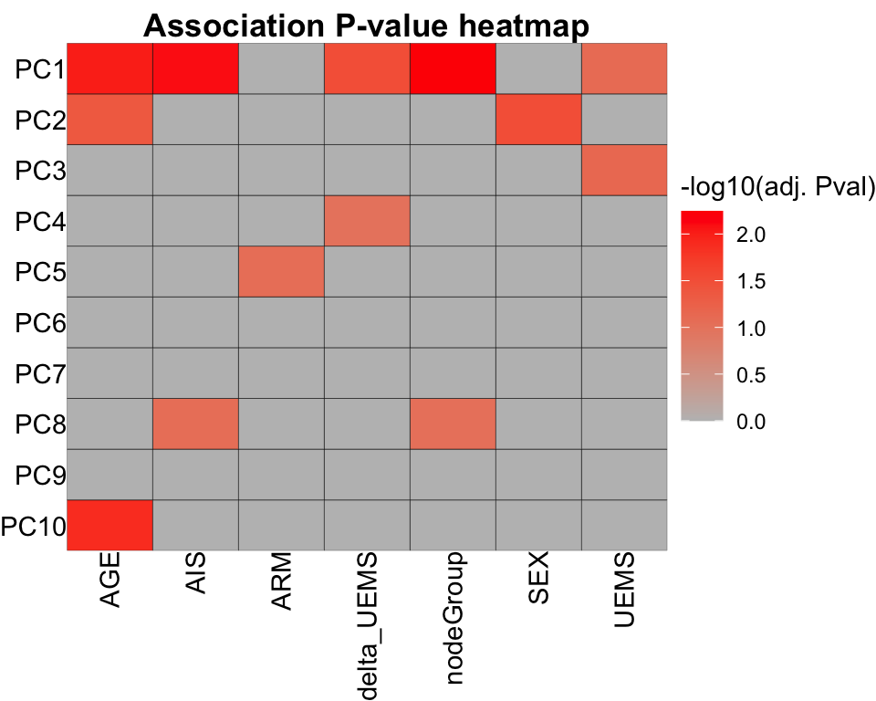
Association between PC1 and nodeGroup
ggplot(plotTab, aes(x=nodeGroup,y=PC1)) +
    geom_boxplot(aes(fill = nodeGroup)) +
    geom_point() +
theme_full 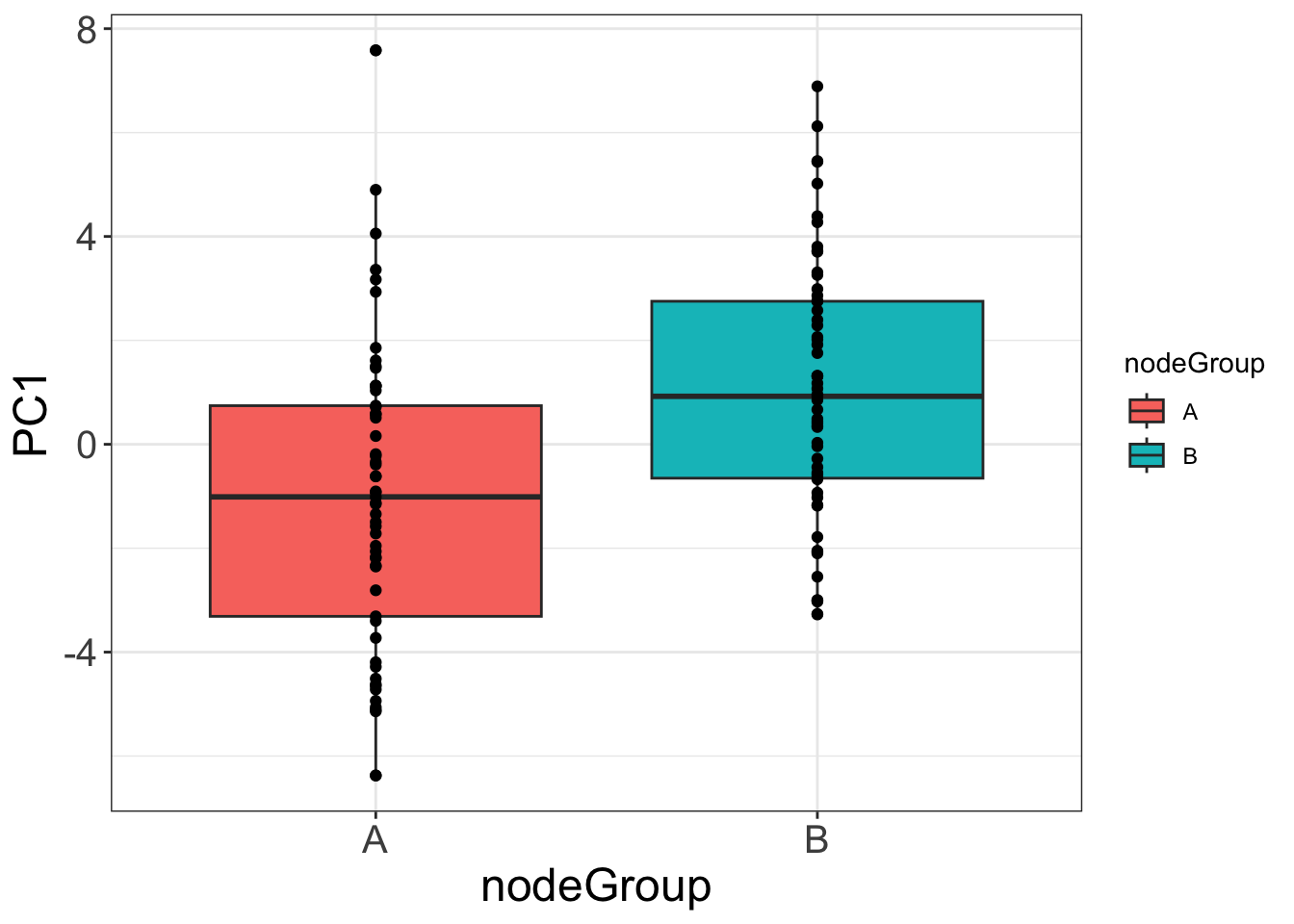
Association between PC1, AIS, node group
ggplot(plotTab, aes(x=AIS,y=PC1)) +
    geom_boxplot(outlier.shape = NA) +
    ggbeeswarm::geom_quasirandom(aes(color = nodeGroup))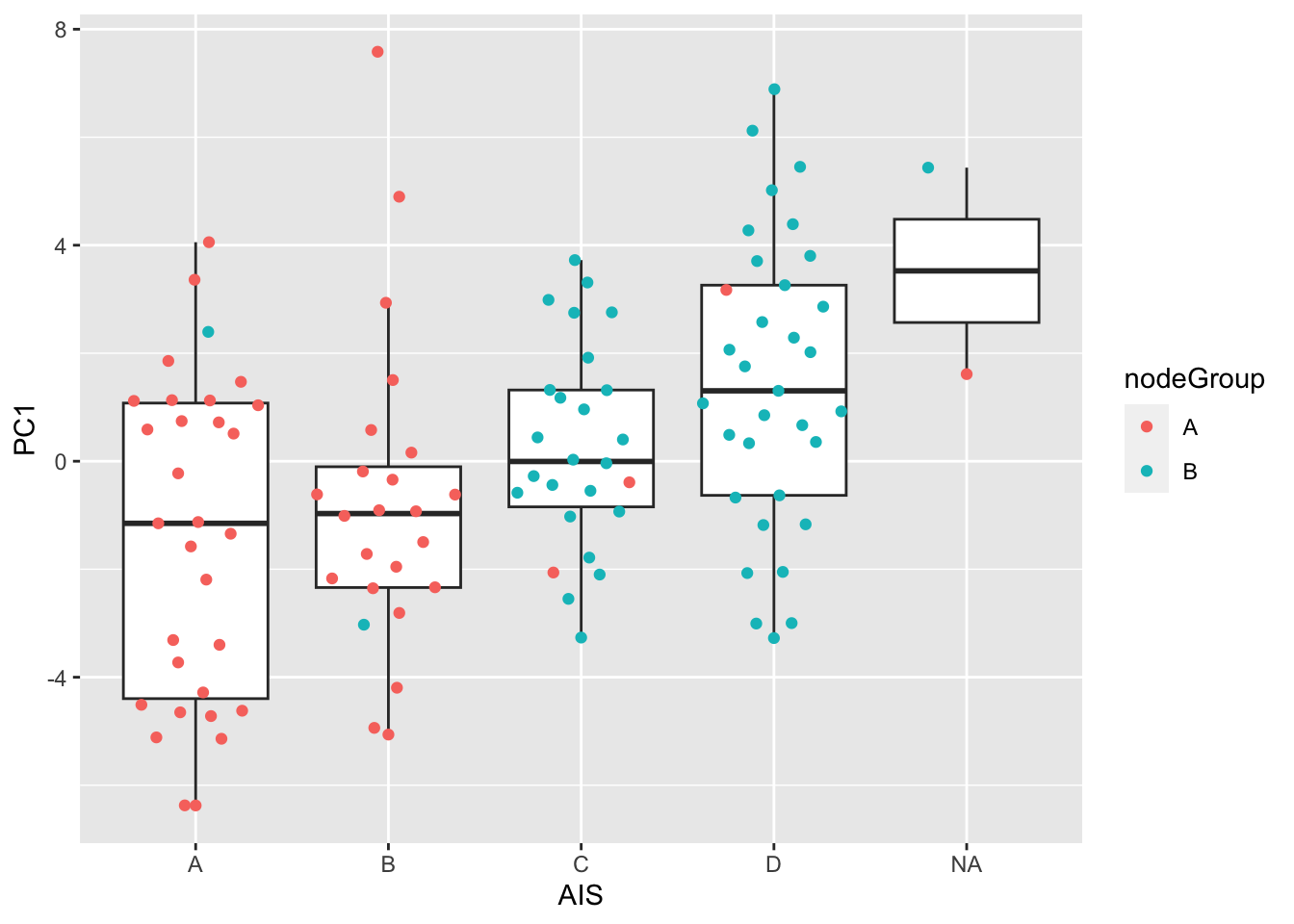
Association between delta_UEMS, treatment and node group
plotTab <- filter(plotTab, !is.na(AIS))
ggplot(plotTab, aes(x=AIS,y=delta_UEMS)) +
    geom_boxplot(outlier.shape = NA) +
    ggbeeswarm::geom_quasirandom(aes(color = nodeGroup)) +
  facet_wrap(~ARM) +
  theme_bw()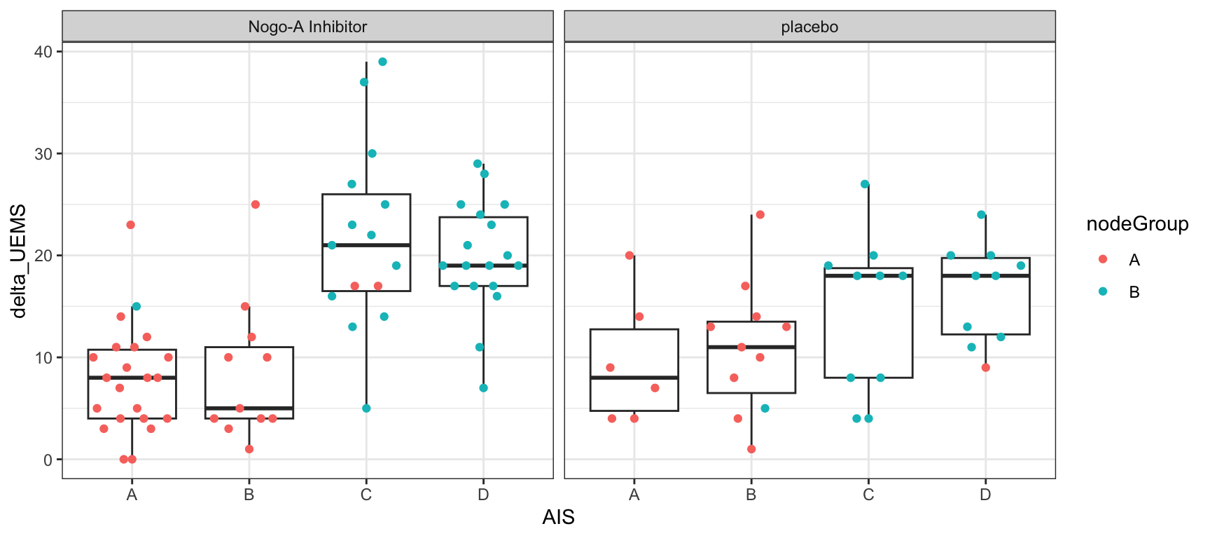
Plots
PC1 versus PC2
ggplot(plotTab, aes(x=PC1, y=PC2, shape = nodeGroup, color = AIS)) +
    geom_point() +
    xlab(sprintf("PC1 (%1.2f%%)",varExp[1])) +
    ylab(sprintf("PC2 (%1.2f%%)",varExp[2])) +
    scale_shape_manual(values=c(A=1, B = 16)) +
    theme_bw()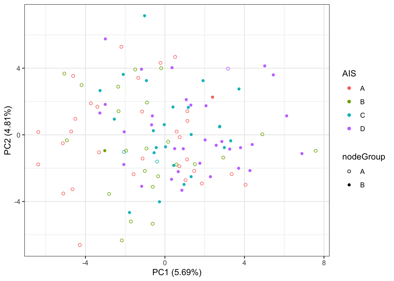
Identify proteins associated with node group in the baseline samples
protSub <- prepareProt(seProt_corr, filterCondi = list(Visit = 3), perNA = 0.5)[1] "Number of proteins: 377, number of samples: 116"Using limma for hypothesis testing
designMat <- model.matrix(~nodeGroup, colData(protSub))
resTab <- testDiff(protSub, designMat, "nodeGroupB", assayName = "imputed")

hist(resTab$pval)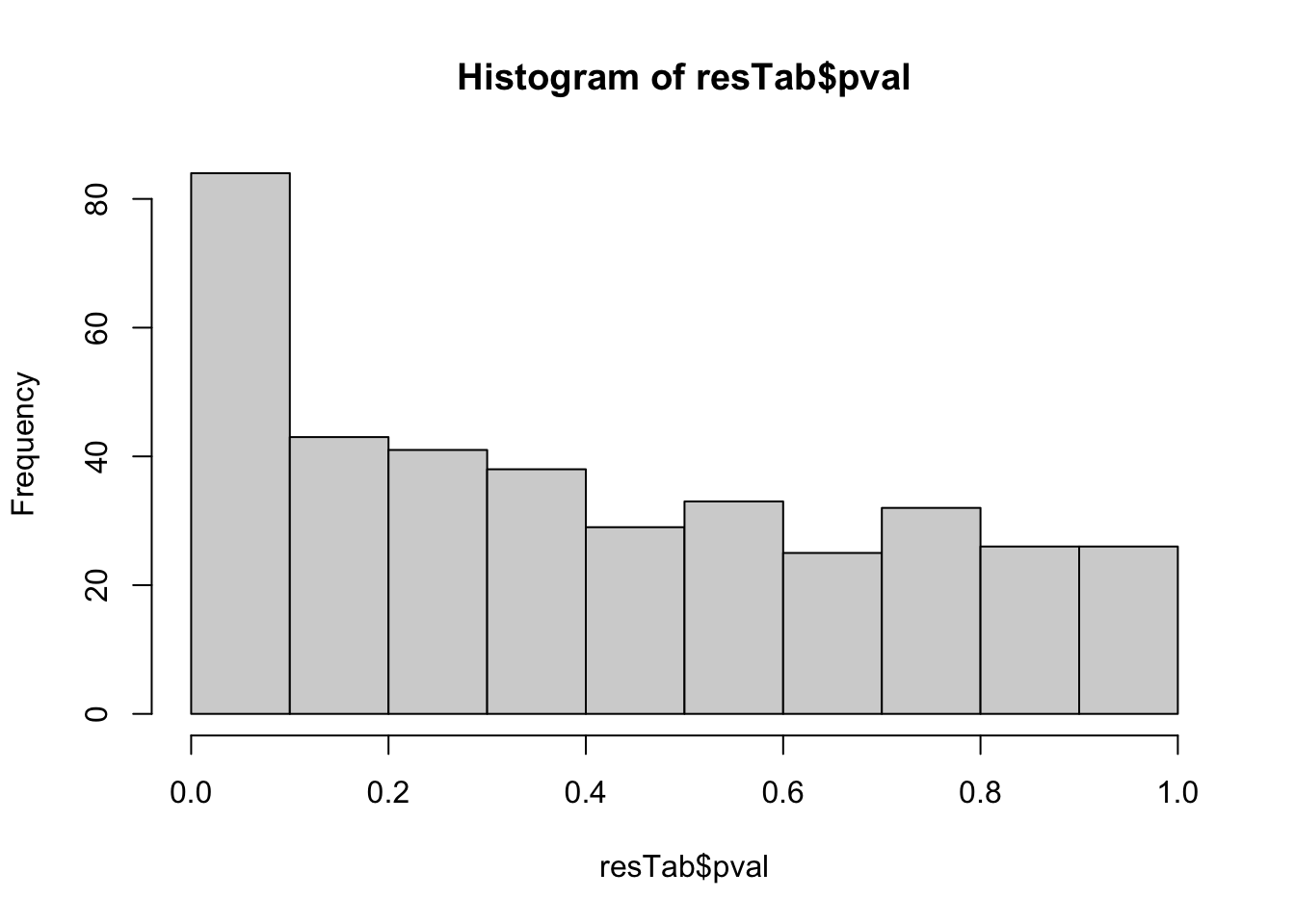
Warning: The above code chunk cached its results, but
it won’t be re-run if previous chunks it depends on are updated. If you
need to use caching, it is highly recommended to also set
knitr::opts_chunk$set(autodep = TRUE) at the top of the
file (in a chunk that is not cached). Alternatively, you can customize
the option dependson for each individual chunk that is
cached. Using either autodep or dependson will
remove this warning. See the
knitr cache options for more details.
List of significant associations
filter(resTab, adj_pval <= 0.25) %>% mutate(across(where(is.numeric), formatC, digits=2)) %>%
  select(name, symbol, pval, adj_pval, diff, n_obs) %>%
  DT::datatable()
Boxplot of top associations
protTab <- jyluMisc::sumToTidy(protSub) %>%
  mutate(ifImputed = ifelse(is.na(count), "yes","no"))

pList <- lapply(seq(9), function(i) {
  rec <- resTab[i,]
  plotTab <- filter(protTab, rowID == rec$name)
  ggplot(plotTab, aes(x=nodeGroup, y = imputed)) +
    geom_boxplot(aes(fill = nodeGroup), outlier.shape = NA)+
    ggbeeswarm::geom_quasirandom(aes(shape = ifImputed)) +
    scale_shape_manual(values = list(yes = 1, no = 16)) +
    ggtitle(sprintf("%s (P=%s)",rec$symbol, formatC(rec$pval, digits = 2))) +
    ylab("Expression") +
    theme_bw() + theme_full + theme(legend.position = "none")
})
cowplot::plot_grid(plotlist = pList, ncol=3)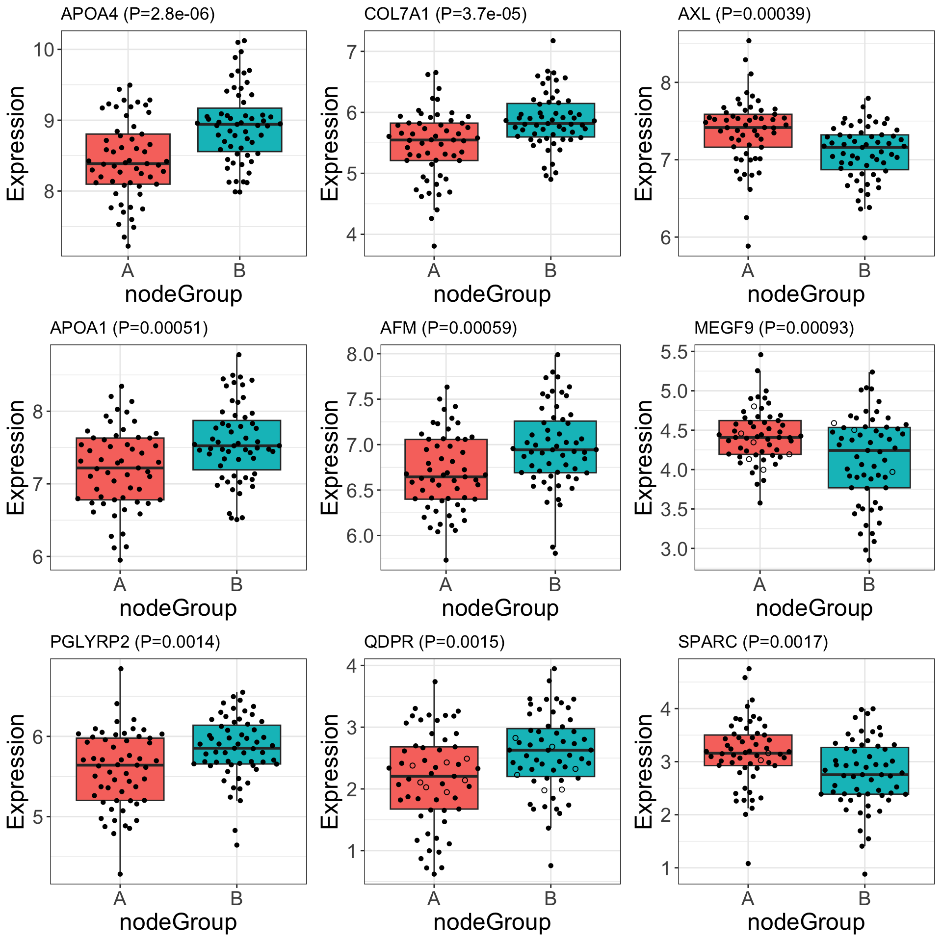
Enrichment analysis
All ranked genes are used. Pathway at 5% FDR level.
gmts = list(GO_BiologicalProcess = "../data/gmts/c5.go.bp.v2023.2.Hs.symbols.gmt",
            GO_MolecularFunction = "../data/gmts/c5.go.mf.v2023.2.Hs.symbols.gmt")
plotList <- runGeneSetEnrichment(resTab, gmts, genePCut  = 1, pCutSet = 0.05, setFdr = FALSE, method = "gsea")
[1] "No sets passed the criteria"plotList$plot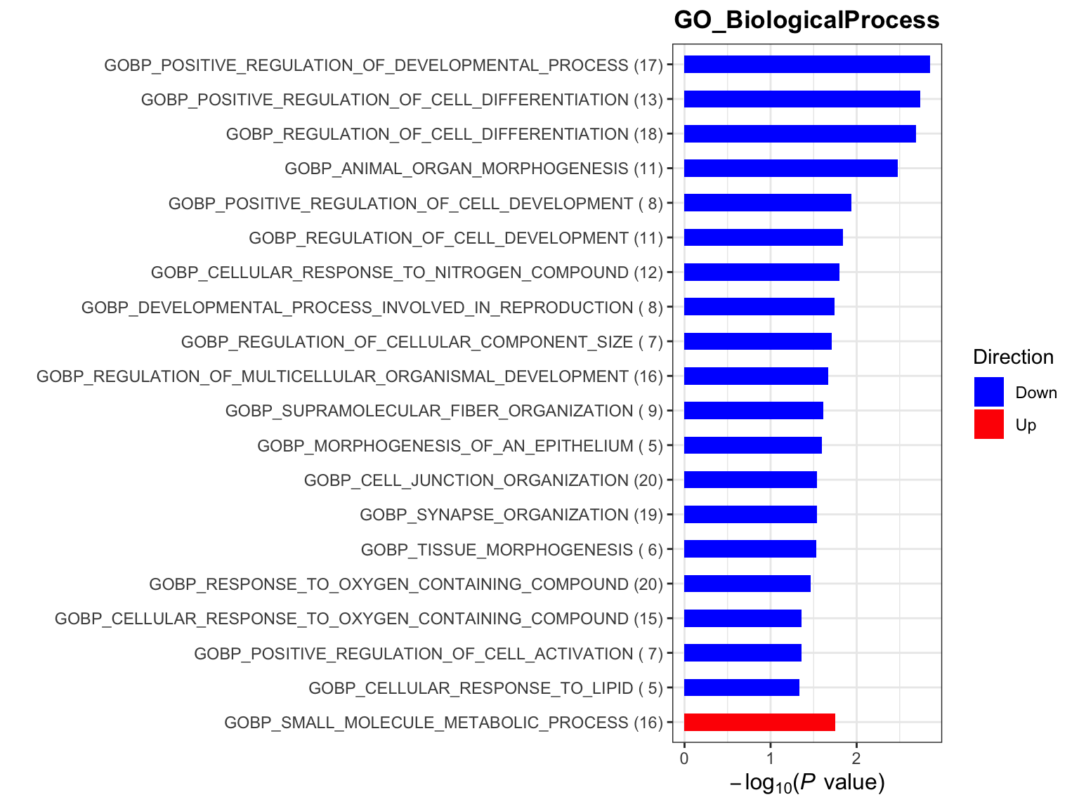
sessionInfo()R version 4.2.0 (2022-04-22)
Platform: x86_64-apple-darwin17.0 (64-bit)
Running under: macOS Big Sur/Monterey 10.16
Matrix products: default
BLAS: /Library/Frameworks/R.framework/Versions/4.2/Resources/lib/libRblas.0.dylib
LAPACK: /Library/Frameworks/R.framework/Versions/4.2/Resources/lib/libRlapack.dylib
locale:
[1] en_US.UTF-8/en_US.UTF-8/en_US.UTF-8/C/en_US.UTF-8/en_US.UTF-8
attached base packages:
[1] stats4 stats graphics grDevices utils datasets methods
[8] base
other attached packages:
[1] forcats_0.5.1 stringr_1.4.1
[3] dplyr_1.1.4.9000 purrr_0.3.4
[5] readr_2.1.2 tidyr_1.2.0
[7] tibble_3.2.1 ggplot2_3.4.1
[9] tidyverse_1.3.2 limma_3.52.2
[11] proDA_1.10.0 SummarizedExperiment_1.26.1
[13] Biobase_2.56.0 GenomicRanges_1.48.0
[15] GenomeInfoDb_1.32.2 IRanges_2.30.0
[17] S4Vectors_0.34.0 BiocGenerics_0.42.0
[19] MatrixGenerics_1.8.1 matrixStats_0.62.0
loaded via a namespace (and not attached):
[1] utf8_1.2.4 shinydashboard_0.7.2 tidyselect_1.2.1
[4] RSQLite_2.2.15 AnnotationDbi_1.58.0 htmlwidgets_1.5.4
[7] grid_4.2.0 BiocParallel_1.30.3 maxstat_0.7-25
[10] munsell_0.5.0 codetools_0.2-18 DT_0.23
[13] withr_3.0.0 colorspace_2.0-3 highr_0.9
[16] knitr_1.39 rstudioapi_0.13 ggsignif_0.6.3
[19] labeling_0.4.2 git2r_0.30.1 slam_0.1-50
[22] GenomeInfoDbData_1.2.8 KMsurv_0.1-5 bit64_4.0.5
[25] farver_2.1.1 rprojroot_2.0.3 vctrs_0.6.5
[28] generics_0.1.3 TH.data_1.1-1 xfun_0.31
[31] sets_1.0-21 R6_2.5.1 ggbeeswarm_0.6.0
[34] locfit_1.5-9.6 bitops_1.0-7 cachem_1.0.6
[37] fgsea_1.22.0 DelayedArray_0.22.0 assertthat_0.2.1
[40] promises_1.2.0.1 scales_1.2.0 multcomp_1.4-19
[43] googlesheets4_1.0.0 beeswarm_0.4.0 gtable_0.3.0
[46] sva_3.44.0 sandwich_3.0-2 workflowr_1.7.0
[49] rlang_1.1.3 genefilter_1.78.0 splines_4.2.0
[52] rstatix_0.7.0 gargle_1.2.0 broom_1.0.0
[55] BiocManager_1.30.18 yaml_2.3.5 abind_1.4-5
[58] modelr_0.1.8 crosstalk_1.2.0 backports_1.4.1
[61] httpuv_1.6.6 tools_4.2.0 relations_0.6-12
[64] ellipsis_0.3.2 gplots_3.1.3 jquerylib_0.1.4
[67] Rcpp_1.0.9 visNetwork_2.1.0 zlibbioc_1.42.0
[70] RCurl_1.98-1.7 ggpubr_0.4.0 cowplot_1.1.1
[73] zoo_1.8-10 haven_2.5.0 cluster_2.1.3
[76] exactRankTests_0.8-35 fs_1.5.2 magrittr_2.0.3
[79] data.table_1.14.8 reprex_2.0.1 survminer_0.4.9
[82] googledrive_2.0.0 mvtnorm_1.1-3 hms_1.1.1
[85] shinyjs_2.1.0 mime_0.12 evaluate_0.15
[88] xtable_1.8-4 XML_3.99-0.10 readxl_1.4.0
[91] gridExtra_2.3 compiler_4.2.0 KernSmooth_2.23-20
[94] crayon_1.5.2 htmltools_0.5.4 mgcv_1.8-40
[97] later_1.3.0 tzdb_0.3.0 lubridate_1.8.0
[100] DBI_1.1.3 dbplyr_2.2.1 MASS_7.3-58
[103] jyluMisc_0.1.5 BiocStyle_2.24.0 Matrix_1.5-4
[106] car_3.1-0 cli_3.6.2 marray_1.74.0
[109] parallel_4.2.0 igraph_1.3.4 pkgconfig_2.0.3
[112] km.ci_0.5-6 piano_2.12.0 xml2_1.3.3
[115] annotate_1.74.0 vipor_0.4.5 bslib_0.4.1
[118] XVector_0.36.0 drc_3.0-1 rvest_1.0.2
[121] digest_0.6.30 Biostrings_2.64.0 rmarkdown_2.14
[124] cellranger_1.1.0 fastmatch_1.1-3 survMisc_0.5.6
[127] edgeR_3.38.1 shiny_1.7.4 gtools_3.9.3
[130] lifecycle_1.0.4 nlme_3.1-158 jsonlite_1.8.3
[133] carData_3.0-5 fansi_1.0.6 pillar_1.9.0
[136] lattice_0.20-45 KEGGREST_1.36.3 fastmap_1.1.0
[139] httr_1.4.3 plotrix_3.8-2 survival_3.4-0
[142] glue_1.7.0 png_0.1-7 bit_4.0.4
[145] stringi_1.7.8 sass_0.4.2 blob_1.2.3
[148] caTools_1.18.2 memoise_2.0.1