Last updated: 2024-05-17

Checks: 5 1

Knit directory: SpinalCord_proteomics/analysis/

This reproducible R Markdown analysis was created with workflowr (version 1.7.0). The Checks tab describes the reproducibility checks that were applied when the results were created. The Past versions tab lists the development history.

Environment: empty

Great job! The global environment was empty. Objects defined in the global environment can affect the analysis in your R Markdown file in unknown ways. For reproduciblity it’s best to always run the code in an empty environment.

Seed: set.seed(20221110)

The command set.seed(20221110) was run prior to running the code in the R Markdown file. Setting a seed ensures that any results that rely on randomness, e.g. subsampling or permutations, are reproducible.

Session information: recorded

Great job! Recording the operating system, R version, and package versions is critical for reproducibility.

Cache: none

Nice! There were no cached chunks for this analysis, so you can be confident that you successfully produced the results during this run.

File paths: relative

Great job! Using relative paths to the files within your workflowr project makes it easier to run your code on other machines.

Repository version: no version control

Tracking code development and connecting the code version to the results is critical for reproducibility. To start using Git, open the Terminal and type git init in your project directory.

This project is not being versioned with Git. To obtain the full reproducibility benefits of using workflowr, please see ?wflow_start.

What are the protein markers that in general change over time?

Subsetting

#subset for patients in the placebo group
protSub <- prepareProt(seProt_corr, filterCondi = list(Treatment = "1"), perNA =0.5, adjustPat = TRUE)

[1] "Number of proteins: 377, number of samples: 202"

#subset for patients with all three time points
pat.complete <- colData(protSub) %>%
    as_tibble() %>% group_by(PSN) %>%
    summarise(n = length(Visit)) %>%
    filter(n>=3)
protSub <- protSub[,protSub$PSN %in% pat.complete$PSN]

print("How many patients?")

[1] "How many patients?"

nrow(pat.complete)

[1] 59

print("How many proteins and samples")

[1] "How many proteins and samples"

dim(protSub)

[1] 377 177

Use spline fitting to identify proteins that change over time.

protMat <- assay(protSub)
designTab <- colData(protSub) %>%
  data.frame()

designTab$X <- splines::ns(designTab$Visit, df=2)

design <- model.matrix(~0 + X + PSN, designTab)
resTab <- testDiff(protSub, design, c("X1","X2"), assayName = "imputed")

Table of proteins passed raw P-value < 0.05

filter(resTab, pval <= 0.05) %>% mutate(across(where(is.numeric), formatC, digits=2)) %>%
  select(name, symbol, pval, adj_pval, n_obs) %>%
  DT::datatable()

Visualize top hits using line plot

exprMat <- assays(protSub)[["imputed"]]
exprMat.patReg <- assays(protSub)[["patReg"]]
pList <- lapply(seq(20), function(i) {
    rec <- resTab[i,]
    plotTab <- tibble(expr = exprMat.patReg[rec$name,],
                      PSN = protSub$PSN,
                      Visit = protSub$Visit,
                      nodeGroup = protSub$nodeGroup)
    ggplot(plotTab, aes(x=factor(Visit), y=expr, group = PSN, color = nodeGroup)) +
        geom_line() +
        geom_point() +
        ggtitle(sprintf("%s (P=%s)",rec$symbol,formatC(rec$pval, digits = 2))) +
        #scale_color_gradient(low="green",high="red") +
        theme_bw() +
        theme(plot.title = element_text(hjust = 0.5, face = "bold")) +
        theme_full +
        xlab("Visit") + ylab("Expression")
})

cowplot::plot_grid(plotlist = pList, ncol=4)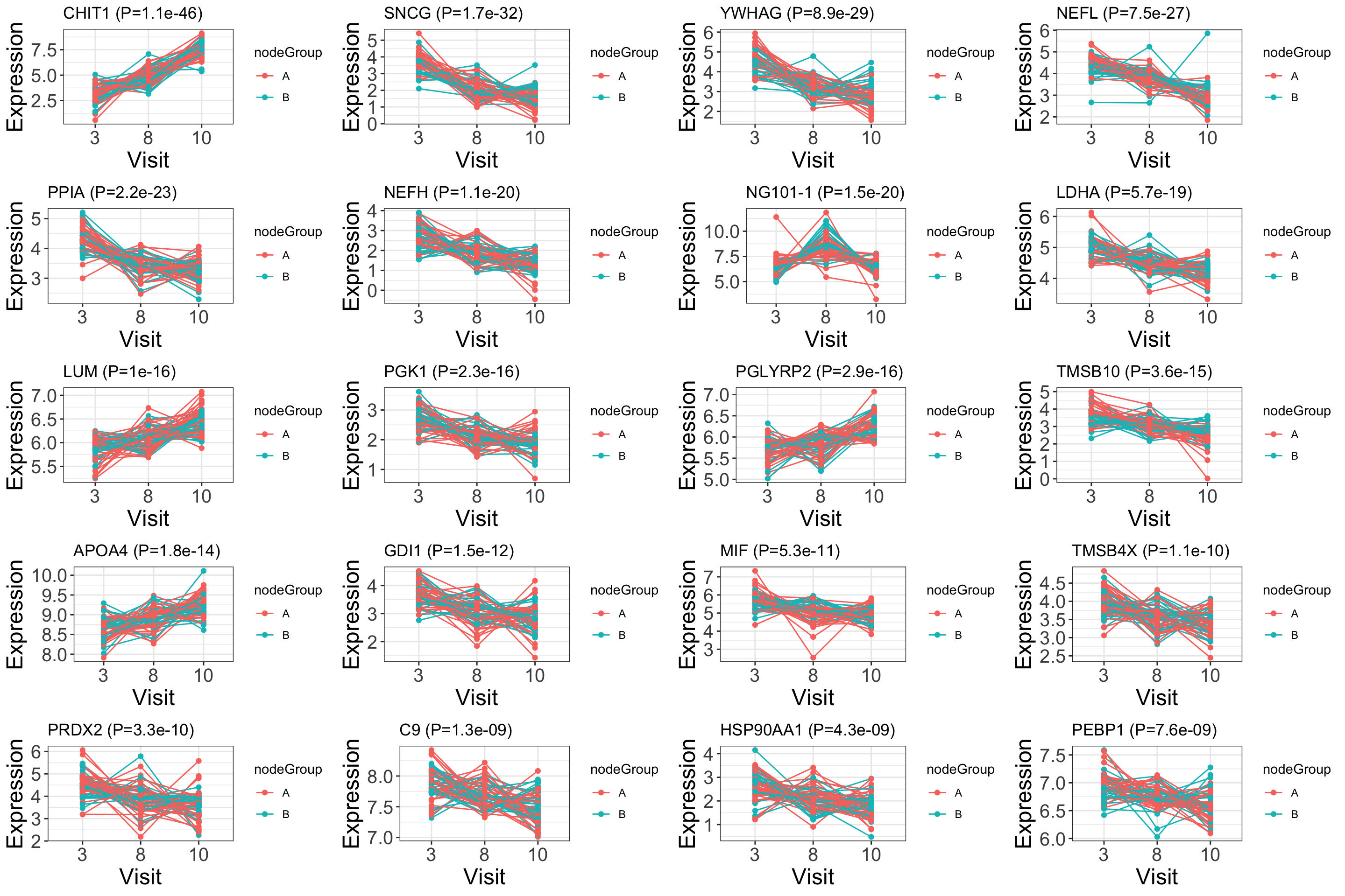

Visualization using heatmap

#need to adjust for patient specific effect first
plotMat <- exprMat.patReg[filter(resTab, adj_pval < 0.1)$name,]

annoCol <- tibble(row = colnames(plotMat),
                  Visit = protSub[,row]$Visit) %>%
    arrange(Visit) %>% 
    mutate(Visit = paste0("V",Visit)) %>%
    column_to_rownames("row") %>% data.frame()
plotMat <- plotMat[,rownames(annoCol)]
pheatmap::pheatmap(plotMat, scale = "row", cluster_rows = TRUE, cluster_cols = FALSE, 
                   color=colorRampPalette(c("navy", "white", "red"))(50),
                   labels_row = rowData(protSub[rownames(plotMat),])$symbol,
                   annotation_col = annoCol, clustering_method = "ward.D2")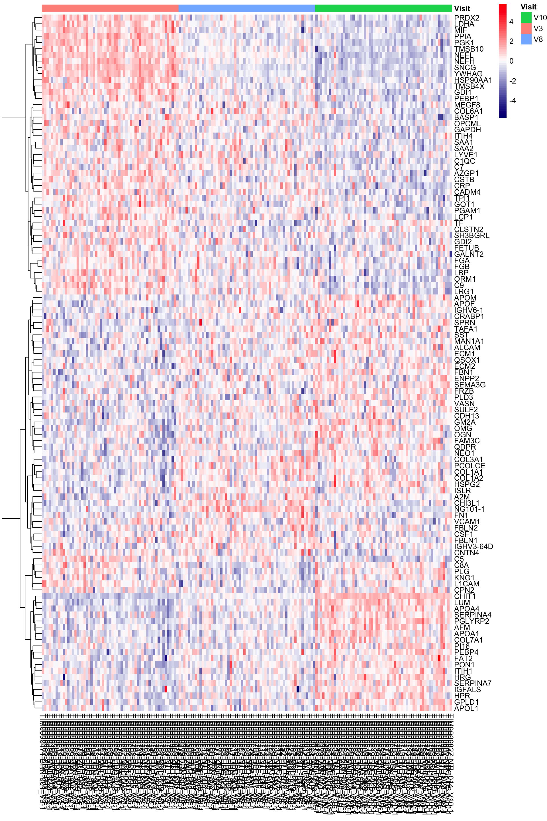

What are the protein markers that change over time and show different trend in the better recovered and worse recovered patients?

Use all three time points

Prepare data

#subset for patients in the placebo group
protSub <- prepareProt(seProt_corr, filterCondi = list(Treatment = "1"), perNA = 0.5, adjustPat = TRUE)

[1] "Number of proteins: 377, number of samples: 202"

#seProt_corr[,seProt_corr$Treatment %in% 0 & !is.na(seProt_corr$delta_UEMS)]

protSub$group_UEMS <- ifelse(protSub$delta_UEMS >= quantile(protSub$delta_UEMS,0.75, na.rm=TRUE), "high", 
                             ifelse(protSub$delta_UEMS <= quantile(protSub$delta_UEMS,0.25, na.rm=TRUE), "low", NA))
protSub <- protSub[,!is.na(protSub$group_UEMS)]

#subset for patients with all three time points
pat.complete <- colData(protSub) %>%
    as_tibble() %>% group_by(PSN) %>%
    summarise(n = length(Visit)) %>%
    filter(n>=3)

protSub <- protSub[,protSub$PSN %in% pat.complete$PSN]

print("How many patients?")

[1] "How many patients?"

nrow(pat.complete)

[1] 27

print("How many proteins and samples")

[1] "How many proteins and samples"

dim(protSub)

[1] 377  81

The high and low delta_UEMS are defined by 75% quantile. The high_UEMS group is the group with better recovery.

Use spline fitting to identify proteins that change overtime.

designTab <- colData(protSub) %>% 
  data.frame()
designTab$X <- splines::ns(designTab$Visit, df=2)

design <- model.matrix(~ group_UEMS + X +  X:group_UEMS, designTab)

resTab <- testDiff(protSub, design, coef = c("group_UEMSlow:X1","group_UEMSlow:X2"), blockID = "PSN", assayName = "imputed")

hist(resTab$pval)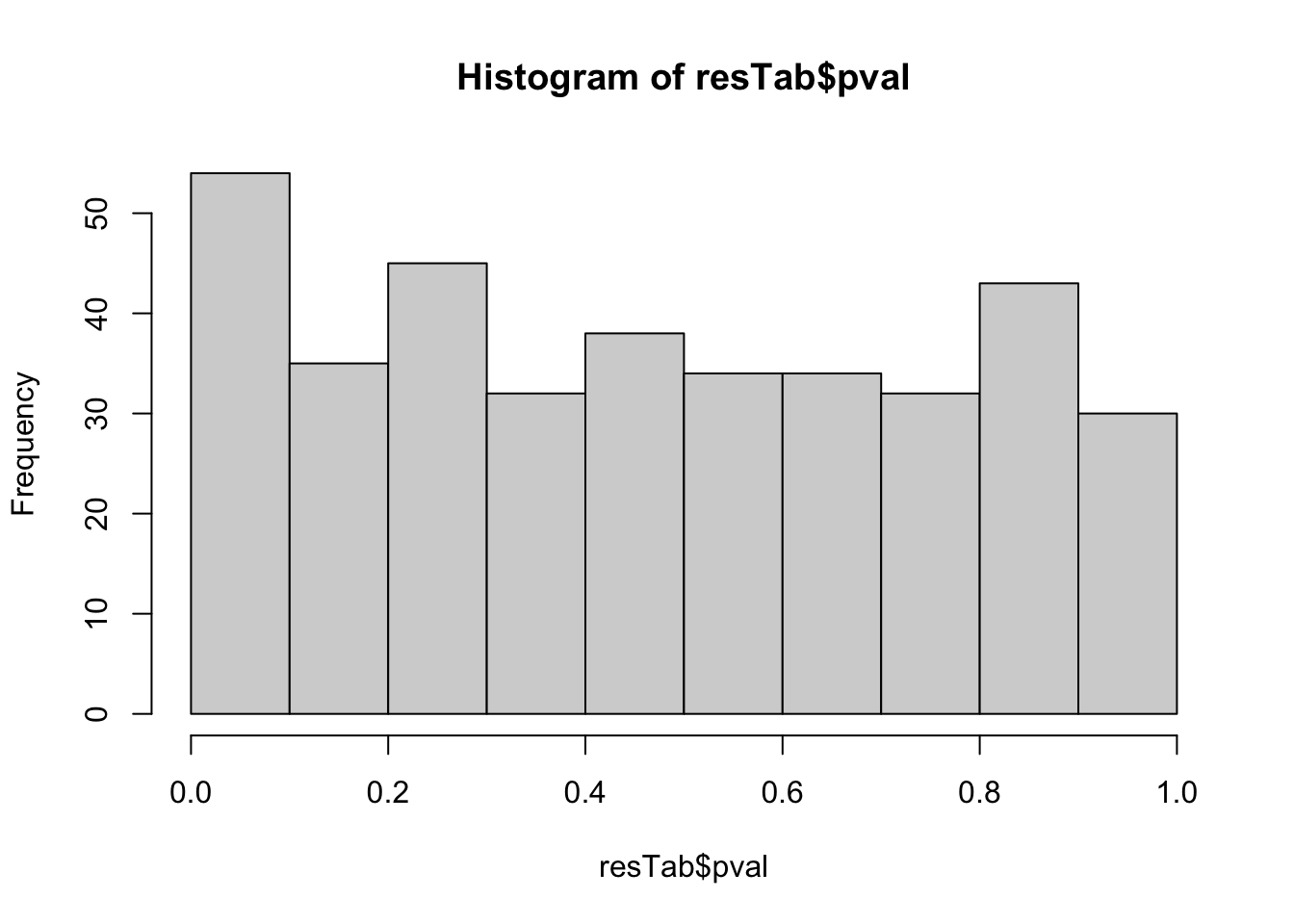

Table of proteins passed raw P-value < 0.05

filter(resTab, pval <= 0.05) %>% mutate(across(where(is.numeric), formatC, digits=2)) %>%
  select(name, symbol, pval, adj_pval, n_obs) %>%
  DT::datatable()

Visualize top hits using line plot

plotDiffTrend(protSub, "group_UEMS")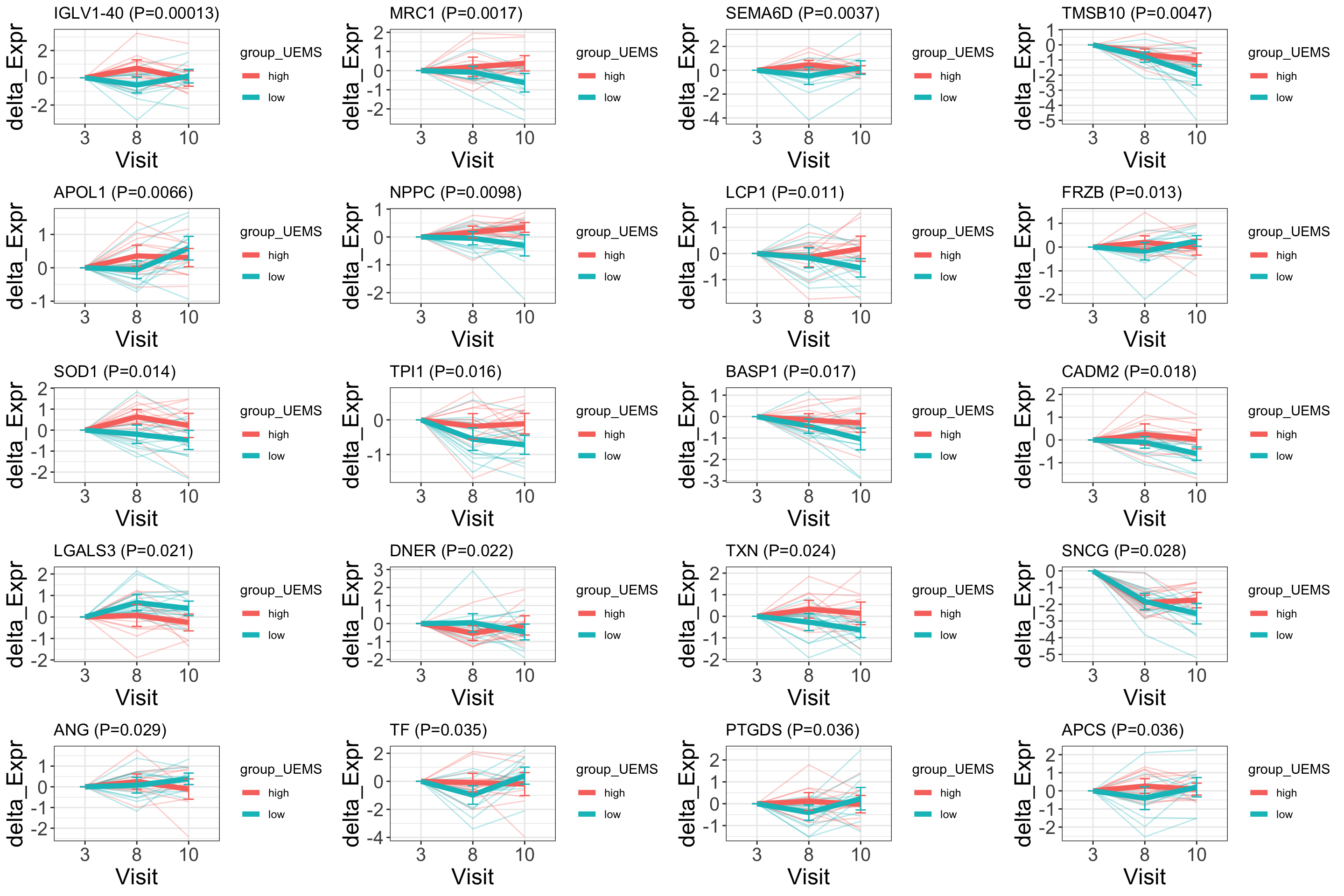

The y-axis shows the expression change to baseline (Visit 3) to better visualize the change

Only look at the first two time points

Subsetting

#subset for patients in the placebo group
protSub <- prepareProt(seProt_corr, filterCondi = list(Treatment = "1", Visit =c(3,8)), perNA = 0.5, adjustPat = TRUE)

[1] "Number of proteins: 378, number of samples: 140"

#seProt_corr[,seProt_corr$Treatment %in% 0 & !is.na(seProt_corr$delta_UEMS)]

protSub$group_UEMS <- ifelse(protSub$delta_UEMS >= quantile(protSub$delta_UEMS,0.75, na.rm=TRUE), "high", 
                             ifelse(protSub$delta_UEMS <= quantile(protSub$delta_UEMS,0.25, na.rm=TRUE), "low", NA))
protSub <- protSub[,!is.na(protSub$group_UEMS)]

#subset for patients with all three time points
pat.complete <- colData(protSub) %>%
    as_tibble() %>% group_by(PSN) %>%
    summarise(n = length(Visit)) %>%
    filter(n>=2)

protSub <- protSub[,protSub$PSN %in% pat.complete$PSN]

print("How many patients?")

[1] "How many patients?"

nrow(pat.complete)

[1] 32

print("How many proteins and samples")

[1] "How many proteins and samples"

dim(protSub)

[1] 378  64

Use spline fitting to identify proteins that change overtime.

design <- model.matrix(~group_UEMS + Visit + Visit:group_UEMS, colData(protSub))

resTab <- testDiff(protSub, design, coef = "group_UEMSlow:Visit", assayName = "imputed", method = "limma", blockID = "PSN")
hist(resTab$pval)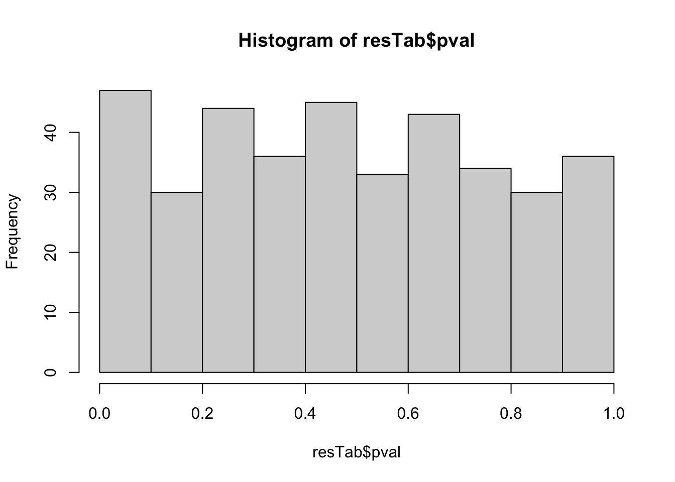

Table of proteins passed raw P-value < 0.05

filter(resTab, pval <= 0.05) %>% mutate(across(where(is.numeric), formatC, digits=2)) %>%
  select(name, symbol, pval, adj_pval, n_obs) %>%
  DT::datatable()

Visualize top hits using line plot

plotDiffTrend(protSub, "group_UEMS")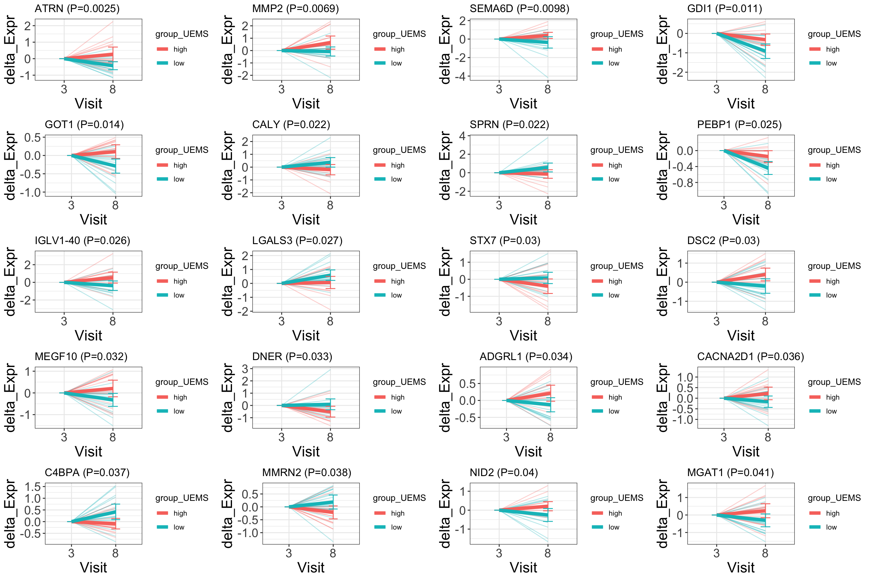

What are the protein markers that change over time and show different trend in the two random node groups, nodeGroup?

Use all three time points

Subsetting

#subset for patients in the placebo group
protSub <- prepareProt(seProt_corr, filterCondi = list(Treatment = "1"), perNA = 0.5, adjustPat = TRUE)

[1] "Number of proteins: 377, number of samples: 202"

#subset for patients with all three time points
pat.complete <- colData(protSub) %>%
    as_tibble() %>% group_by(PSN) %>%
    summarise(n = length(Visit)) %>%
    filter(n>=3)

protSub <- protSub[,protSub$PSN %in% pat.complete$PSN]

print("How many patients?")

[1] "How many patients?"

nrow(pat.complete)

[1] 59

print("How many proteins and samples")

[1] "How many proteins and samples"

dim(protSub)

[1] 377 177

Use spline fitting to identify proteins that change overtime.

designTab <- colData(protSub) %>% 
  data.frame()
designTab$X <- splines::ns(designTab$Visit, df=2)

design <- model.matrix(~ nodeGroup + X +  X:nodeGroup, designTab)

resTab <- testDiff(protSub, design, coef = c("nodeGroupB:X1","nodeGroupB:X2"), blockID = "PSN", assayName = "imputed")

hist(resTab$pval)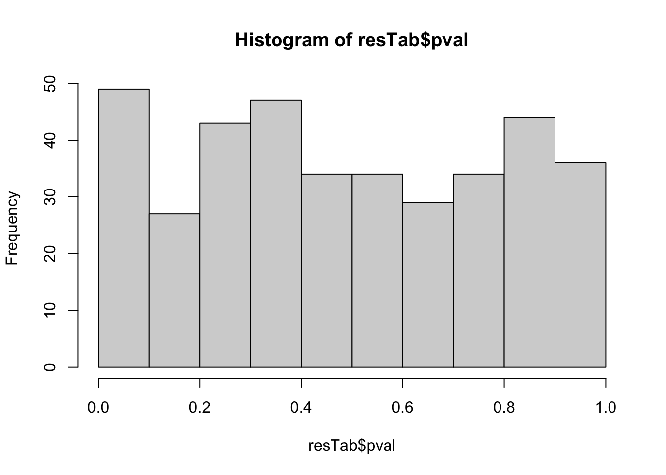

Table of proteins passed raw P-value < 0.05

filter(resTab, pval <= 0.05) %>% mutate(across(where(is.numeric), formatC, digits=2)) %>%
  select(name, symbol, pval, adj_pval, n_obs) %>%
  DT::datatable()

Visualize top hits using line plot

plotDiffTrend(protSub, "nodeGroup")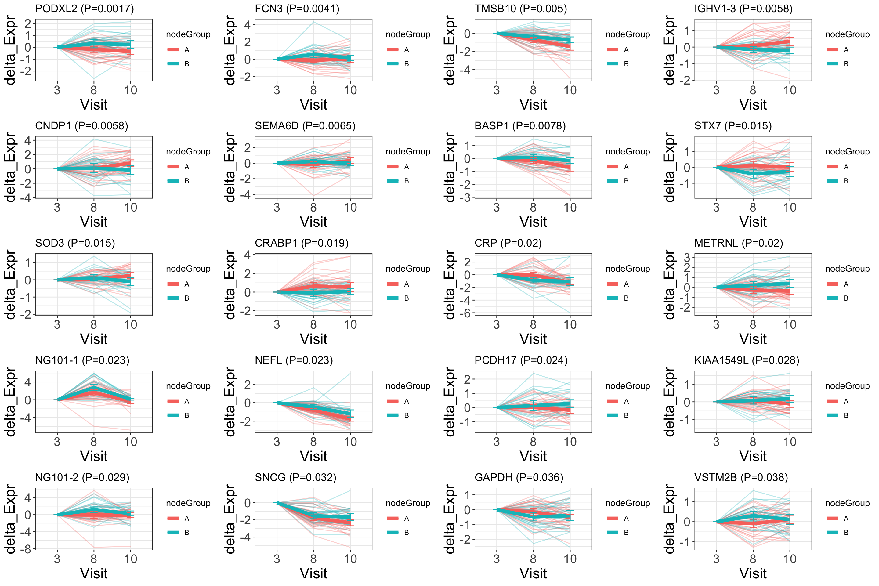

Only look at the first two time points

Subsetting

#subset for patients in the placebo group
protSub <- prepareProt(seProt, filterCondi = list(Treatment = "1", Visit =c(3,8)), perNA = 0.8, adjustPat = TRUE)

[1] "Number of proteins: 428, number of samples: 140"

#subset for patients with all three time points
pat.complete <- colData(protSub) %>%
    as_tibble() %>% group_by(PSN) %>%
    summarise(n = length(Visit)) %>%
    filter(n>=2)

protSub <- protSub[,protSub$PSN %in% pat.complete$PSN]

print("How many patients?")

[1] "How many patients?"

nrow(pat.complete)

[1] 66

print("How many proteins and samples")

[1] "How many proteins and samples"

dim(protSub)

[1] 428 132

Use spline fitting to identify proteins that change overtime.

design <- model.matrix(~nodeGroup + Visit + Visit:nodeGroup, colData(protSub))

resTab <- testDiff(protSub, design, coef = "nodeGroupB:Visit", assayName = "imputed", method = "limma", blockID = "PSN")
hist(resTab$pval)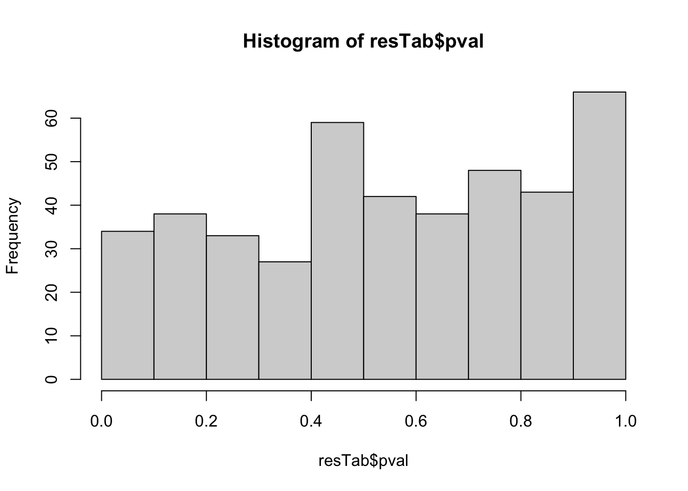

Table of proteins passed raw P-value < 0.05

filter(resTab, pval <= 0.05) %>% mutate(across(where(is.numeric), formatC, digits=2)) %>%
  select(name, symbol, pval, adj_pval, n_obs) %>%
  DT::datatable()

Visualize top hits using line plot

plotDiffTrend(protSub, "nodeGroup")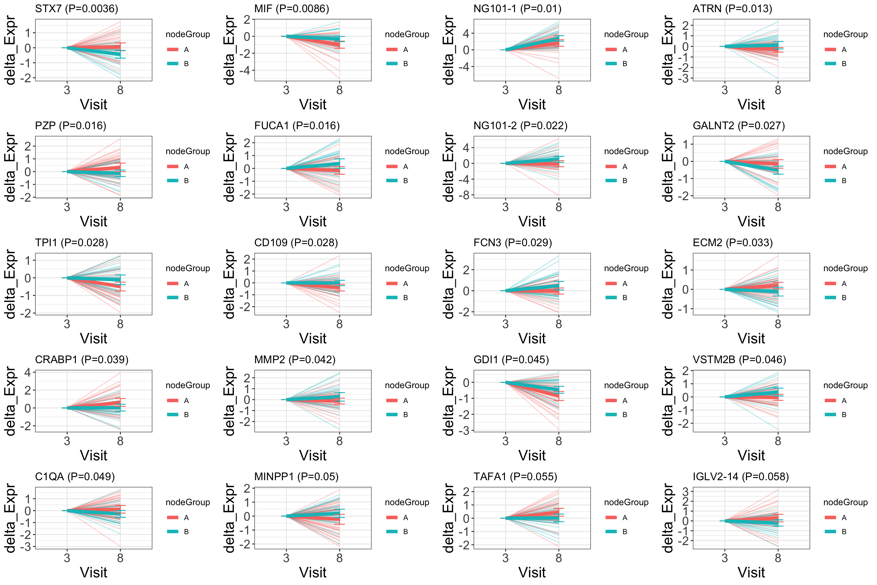

sessionInfo()

R version 4.2.0 (2022-04-22)
Platform: x86_64-apple-darwin17.0 (64-bit)
Running under: macOS Big Sur/Monterey 10.16

Matrix products: default
BLAS:   /Library/Frameworks/R.framework/Versions/4.2/Resources/lib/libRblas.0.dylib
LAPACK: /Library/Frameworks/R.framework/Versions/4.2/Resources/lib/libRlapack.dylib

locale:
[1] en_US.UTF-8/en_US.UTF-8/en_US.UTF-8/C/en_US.UTF-8/en_US.UTF-8

attached base packages:
[1] stats4    stats     graphics  grDevices utils     datasets  methods  
[8] base     

other attached packages:
 [1] forcats_0.5.1               stringr_1.4.1              
 [3] dplyr_1.1.4.9000            purrr_0.3.4                
 [5] readr_2.1.2                 tidyr_1.2.0                
 [7] tibble_3.2.1                ggplot2_3.4.1              
 [9] tidyverse_1.3.2             limma_3.52.2               
[11] proDA_1.10.0                SummarizedExperiment_1.26.1
[13] Biobase_2.56.0              GenomicRanges_1.48.0       
[15] GenomeInfoDb_1.32.2         IRanges_2.30.0             
[17] S4Vectors_0.34.0            BiocGenerics_0.42.0        
[19] MatrixGenerics_1.8.1        matrixStats_0.62.0         

loaded via a namespace (and not attached):
 [1] bitops_1.0-7           fs_1.5.2               lubridate_1.8.0       
 [4] RColorBrewer_1.1-3     httr_1.4.3             rprojroot_2.0.3       
 [7] tools_4.2.0            backports_1.4.1        bslib_0.4.1           
[10] DT_0.23                utf8_1.2.4             R6_2.5.1              
[13] DBI_1.1.3              colorspace_2.0-3       withr_3.0.0           
[16] tidyselect_1.2.1       compiler_4.2.0         git2r_0.30.1          
[19] rvest_1.0.2            cli_3.6.2              xml2_1.3.3            
[22] DelayedArray_0.22.0    labeling_0.4.2         sass_0.4.2            
[25] scales_1.2.0           digest_0.6.30          rmarkdown_2.14        
[28] XVector_0.36.0         pkgconfig_2.0.3        htmltools_0.5.4       
[31] highr_0.9              dbplyr_2.2.1           fastmap_1.1.0         
[34] htmlwidgets_1.5.4      rlang_1.1.3            readxl_1.4.0          
[37] rstudioapi_0.13        farver_2.1.1           jquerylib_0.1.4       
[40] generics_0.1.3         jsonlite_1.8.3         crosstalk_1.2.0       
[43] googlesheets4_1.0.0    RCurl_1.98-1.7         magrittr_2.0.3        
[46] GenomeInfoDbData_1.2.8 Matrix_1.5-4           Rcpp_1.0.9            
[49] munsell_0.5.0          fansi_1.0.6            lifecycle_1.0.4       
[52] stringi_1.7.8          yaml_2.3.5             zlibbioc_1.42.0       
[55] grid_4.2.0             promises_1.2.0.1       crayon_1.5.2          
[58] lattice_0.20-45        cowplot_1.1.1          splines_4.2.0         
[61] haven_2.5.0            hms_1.1.1              knitr_1.39            
[64] pillar_1.9.0           reprex_2.0.1           glue_1.7.0            
[67] evaluate_0.15          BiocManager_1.30.18    modelr_0.1.8          
[70] vctrs_0.6.5            tzdb_0.3.0             httpuv_1.6.6          
[73] cellranger_1.1.0       gtable_0.3.0           assertthat_0.2.1      
[76] cachem_1.0.6           xfun_0.31              broom_1.0.0           
[79] later_1.3.0            googledrive_2.0.0      gargle_1.2.0          
[82] pheatmap_1.0.12        workflowr_1.7.0        statmod_1.4.36        
[85] ellipsis_0.3.2         BiocStyle_2.24.0

Time series analysis on the treated group

Junyan Lu

17 May 2024

What are the protein markers that in general change over time?

Use spline fitting to identify proteins that change over time.

Table of proteins passed raw P-value < 0.05

Visualize top hits using line plot

Visualization using heatmap

What are the protein markers that change over time and show different trend in the better recovered and worse recovered patients?

Use all three time points

Use spline fitting to identify proteins that change overtime.

Table of proteins passed raw P-value < 0.05

Visualize top hits using line plot

Only look at the first two time points

Use spline fitting to identify proteins that change overtime.

Table of proteins passed raw P-value < 0.05

Visualize top hits using line plot

What are the protein markers that change over time and show different trend in the two random node groups, nodeGroup?

Use all three time points

Use spline fitting to identify proteins that change overtime.

Table of proteins passed raw P-value < 0.05

Visualize top hits using line plot

Only look at the first two time points

Use spline fitting to identify proteins that change overtime.

Table of proteins passed raw P-value < 0.05

Visualize top hits using line plot