Build machine learning model for predicting treatment outcome, delta_UEMS

workflowr

• Summary
• Checks
• Past versions

Last updated: 2024-05-17

Checks: 5 1

Knit directory: SpinalCord_proteomics/analysis/

This reproducible R Markdown analysis was created with workflowr (version 1.7.0). The Checks tab describes the reproducibility checks that were applied when the results were created. The Past versions tab lists the development history.

---

Environment: empty

Great job! The global environment was empty. Objects defined in the global environment can affect the analysis in your R Markdown file in unknown ways. For reproduciblity it’s best to always run the code in an empty environment.

Seed: set.seed(20221110)

The command set.seed(20221110) was run prior to running the code in the R Markdown file. Setting a seed ensures that any results that rely on randomness, e.g. subsampling or permutations, are reproducible.

Session information: recorded

Great job! Recording the operating system, R version, and package versions is critical for reproducibility.

Cache: none

Nice! There were no cached chunks for this analysis, so you can be confident that you successfully produced the results during this run.

File paths: relative

Great job! Using relative paths to the files within your workflowr project makes it easier to run your code on other machines.

Repository version: no version control

Tracking code development and connecting the code version to the results is critical for reproducibility. To start using Git, open the Terminal and type git init in your project directory.

---

This project is not being versioned with Git. To obtain the full reproducibility benefits of using workflowr, please see ?wflow_start.

---

Preparing dataset

Subset and removed unwanted variations

Subset

seSub <- prepareProt(seProt, filterCondi = list(Treatment = "1"), perNA = 1)

[1] "Number of proteins: 473, number of samples: 184"

sva

mod <- model.matrix(~ Visit + AIS + UEMS + delta_UEMS + nodeGroup, colData(seSub))
exprMat <- assays(seSub)[[2]]
svaObj <- sva::sva(exprMat, mod)

Number of significant surrogate variables is:  10 
Iteration (out of 5 ):1  2  3  4  5  

assays(seSub)[[1]] <- limma::removeBatchEffect(assay(seSub), covariates = svaObj$sv)
assays(seSub)[[2]] <- limma::removeBatchEffect(assays(seSub)[[2]], covariates = svaObj$sv)

Prepare each proteomic dataset for comparing

Data set for individual time point

protV3 <- prepareProt(seProt, filterCondi = list(Treatment = "1", Visit = 3), perNA = 0.5)

[1] "Number of proteins: 378, number of samples: 66"

colnames(protV3) <- protV3$PSN
protV8 <- prepareProt(seProt, filterCondi = list(Treatment = "1", Visit = 8), perNA = 0.5)

[1] "Number of proteins: 374, number of samples: 61"

colnames(protV8) <- protV8$PSN
protV10 <- prepareProt(seProt, filterCondi = list(Treatment = "1", Visit = 10), perNA = 0.5)

[1] "Number of proteins: 374, number of samples: 57"

colnames(protV10) <- protV10$PSN

Calculate the protein expression difference before and after treatment (V8-V3)

overPat <- intersect(protV8$PSN, protV3$PSN)
overProt <- intersect(rownames(protV3), rownames(protV8))
protSub.before <- protV3[overProt,match(overPat, protV3$PSN)]
protSub.after <- protV8[overProt,match(overPat, protV8$PSN)]
colnames(protSub.after) <- overPat
colnames(protSub.before) <- overPat

protDiff38 <- protSub.before
assays(protDiff38)[[1]] <- assays(protSub.after)[[1]] - assays(protSub.before)[[1]]
assays(protDiff38)[[2]] <- assays(protSub.after)[[2]] - assays(protSub.before)[[2]]

#remove feature with too many missings
#protSub <- protSub[rowSums(is.na(assay(protSub)))/ncol(protSub) < 0.5,]

print("How many proteins and samples")

[1] "How many proteins and samples"

dim(protDiff38)

[1] 372  61

Generate training dataset

For individual data, pre-filtering by association test, raw P < 0.1, to reduce the dimentions

pCut = 0.05
allTrainData <- list(
  V3 = list(y = protV3$delta_UEMS,
            X = assays(protV3)[[2]][rownames(protV3) %in% filter(allResList$corrOutcome_baseline_treated, pval <= pCut)$symbol,]),
  V8 = list(y = protV8$delta_UEMS,
            X = assays(protV8)[[2]][rownames(protV8) %in% filter(allResList$corrOutcome_visit8_treated, pval <= pCut)$symbol,]),
  #V10 = list(y = protV10$delta_UEMS,
   #         X = assays(protV10)[[2]][rownames(protV10) %in% filter(allResList$corrOutcome_visit10_treated, pval <= pCut)$symbol,]),
  diff38 = list(y = protDiff38$delta_UEMS,
            X = assays(protDiff38)[[2]][rownames(protDiff38) %in% filter(allResList$corrOutcome_diff83_treated, pval <= pCut)$symbol,])
)

Combined data

overPat <- jyluMisc::overlap(colnames(protV3), colnames(protV8), colnames(protV10), colnames(protDiff38))
comMat <- lapply(names(allTrainData), function(n) {
  exprMat <- allTrainData[[n]]$X[,overPat]
  rownames(exprMat) <- paste0(n,"_",rownames(exprMat))
  exprMat
}) %>% do.call(rbind,.)
allTrainData[["combine"]] <- list(y = protDiff38[,overPat]$delta_UEMS, X = comMat[,overPat])

Use random lasso to rank features by their importance

source("../code/Random_lasso.R")

Calculate feature importance patth by random lasso

set.seed(2024)
rndLassoRes <- list()
rndRes <- lapply(names(allTrainData), function(n) {
  X <- scale(t(allTrainData[[n]]$X))
  y <- allTrainData[[n]]$y
  res <- featurePath(X, y, sampleFraction = 0.5, weakness =0.2, nPerm = 1000, 
                        typePerm = "standard", lambda = seq(1,0.01,length.out = 100))
  tibble(feature = rownames(res$freqMat),
         importance = rowMeans(res$freqMat),
         set = n)
}) %>% bind_rows()

Warning: The above code chunk cached its results, but it won’t be re-run if previous chunks it depends on are updated. If you need to use caching, it is highly recommended to also set knitr::opts_chunk$set(autodep = TRUE) at the top of the file (in a chunk that is not cached). Alternatively, you can customize the option dependson for each individual chunk that is cached. Using either autodep or dependson will remove this warning. See the knitr cache options for more details.

List of the top 30 most important features

pList <- lapply(unique(rndRes$set), function(s) {
  eachTab <- filter(rndRes, set == s) %>%
    arrange(desc(importance)) %>%
    slice_head(n=30) %>%
    mutate(feature = factor(feature, levels = feature))
  ggplot(eachTab, aes(x=feature, y=importance)) +
    geom_bar(stat ="identity") +
    ggtitle(s) +
    theme_bw() +
    theme(axis.text.x = element_text(angle = 90, hjust = 1, vjust = 0),
          plot.title = element_text(face ="bold", size=10, hjust = 0.5))
})
cowplot::plot_grid(plotlist= pList, ncol=1)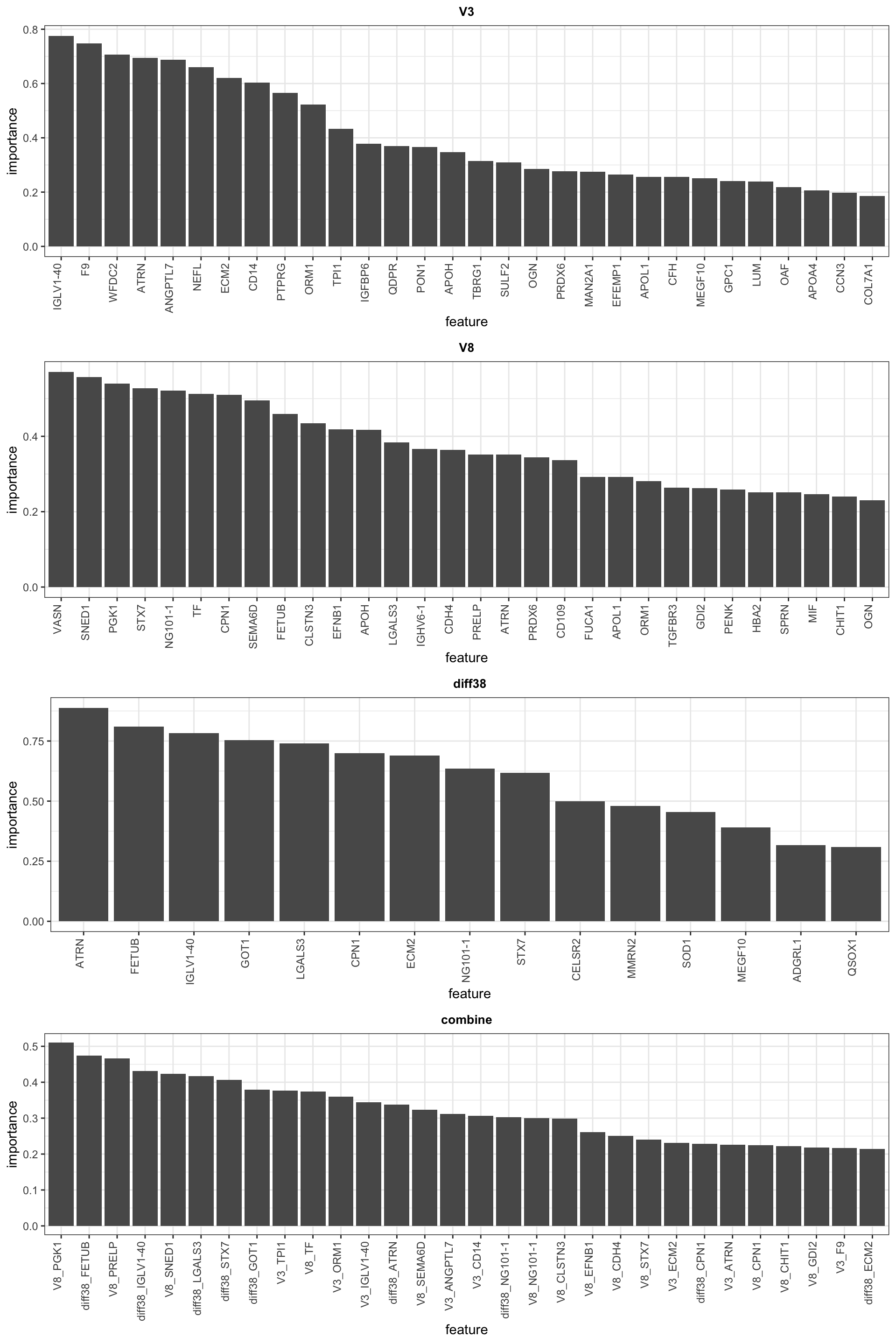

Test the performance of using different number of features

set.seed(2024)
featureNum <- c(3,5, seq(10,20),30)

allCompareRes <- lapply(unique(names(allTrainData)), function(n) {
  eachCompareRes <- lapply(featureNum, function(m) {
      seleFeature <- filter(rndRes, set == n) %>%
        slice_max(importance, n=m) %>% pull(feature)
      X <- scale(t(allTrainData[[n]]$X))[,seleFeature]
      y <- allTrainData[[n]]$y
      
      perf <- testModel(X, y, repeats = 100, testRatio = 0.3)
      
      tibble(set = n, num = m, 
             meanR2 = mean(perf, na.rm=TRUE),
             sdR2 = sd(perf, na.rm=TRUE),
             CI = 1.96*sdR2/sqrt(length(perf)))
  }) %>% bind_rows()
}) %>% bind_rows()

Warning: The above code chunk cached its results, but it won’t be re-run if previous chunks it depends on are updated. If you need to use caching, it is highly recommended to also set knitr::opts_chunk$set(autodep = TRUE) at the top of the file (in a chunk that is not cached). Alternatively, you can customize the option dependson for each individual chunk that is cached. Using either autodep or dependson will remove this warning. See the knitr cache options for more details.

ggplot(allCompareRes, aes(x=factor(num), y=meanR2, fill = set)) +
  geom_bar(stat="identity") +
  geom_errorbar(aes(ymax = meanR2 + CI, ymin = meanR2-CI), width=0.5) +
  facet_wrap(~set, scale = "free_x") +
  theme(legend.position = "none") +
  xlab("Number of protein markers") + ylab("Variance explained") +
  theme_bw() + theme(legend.position = "none")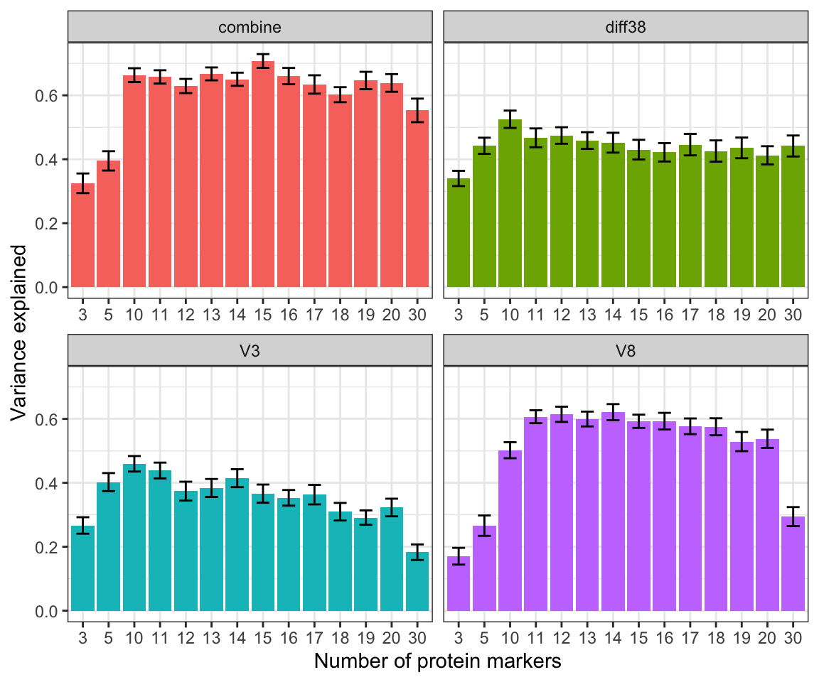

The higher variance explained, the better the models are This graph shows that the best performing model are 1) Using 15 proteins from the combined V3 and V8 proteomics. 2) Using proteins from the V8 proteomic dataset (slightly worse than the first mdoel) If we only want to use the baseline for prediction, 10 features from the V3 dataset performs the best

Visualize the 15 features from the combined dataset

seleFeature <- filter(rndRes, set == "combine") %>%
    slice_max(importance, n=15) %>% pull(feature)

#predict the score
scoreList <- list()
X <- t(allTrainData[["combine"]]$X)[,seleFeature]
y <- allTrainData[["combine"]]$y
seleModel <- glmnet(X, y, lambda =0)
y.pred <- predict(seleModel, newx = X)[,1]
scoreList[["combine_15"]] <- y.pred


plotMat <- allTrainData$combine$X[seleFeature,]
annoCol <- data.frame(row.names = colnames(plotMat), delta_UEMS = allTrainData$combine$y, 
                      proteinScore = y.pred,
                      nodeGroup = protDiff38[,colnames(plotMat)]$nodeGroup)
annoCol <- annoCol[order(annoCol$delta_UEMS),,drop=FALSE]
plotMat <- plotMat[,rownames(annoCol)]
pheatmap::pheatmap(plotMat, annotation_col = annoCol, cluster_rows = TRUE, cluster_cols = FALSE, scale = "row",
                   clustering_method = "ward.D2",
                   color = colorRampPalette(c("blue", "white", "red"))(100))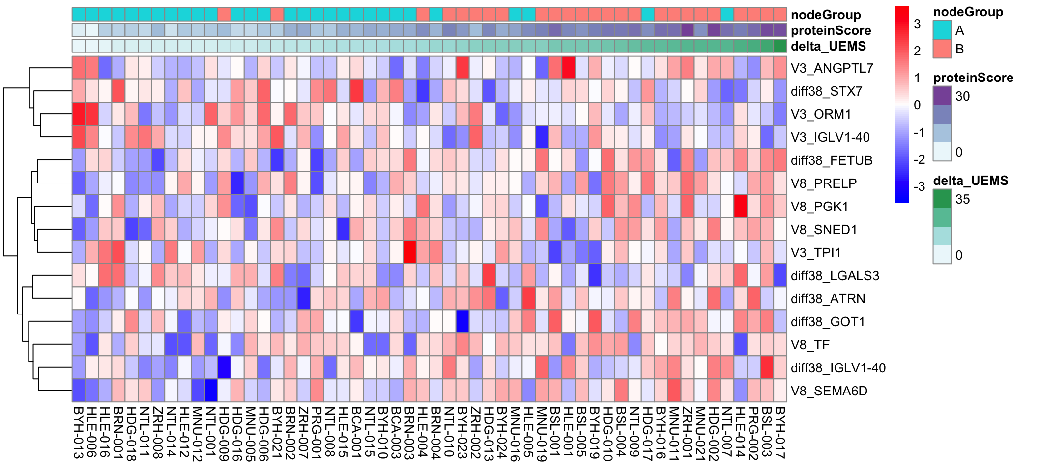

Visualize the 14 features from the V8 dataset

seleFeature <- filter(rndRes, set == "V8") %>%
    slice_max(importance, n=14) %>% pull(feature)

#predict the score
X <- t(allTrainData[["V8"]]$X)[,seleFeature]
y <- allTrainData[["V8"]]$y
seleModel <- glmnet(X, y, lambda =0)
y.pred <- predict(seleModel, newx = X)[,1]
scoreList[["V8_14"]] <- y.pred


plotMat <- allTrainData$V8$X[seleFeature,]
annoCol <- data.frame(row.names = colnames(plotMat), delta_UEMS = allTrainData$V8$y, 
                      proteinScore = y.pred,
                      nodeGroup = protV8[,colnames(plotMat)]$nodeGroup)
annoCol <- annoCol[order(annoCol$delta_UEMS),,drop=FALSE]
plotMat <- plotMat[,rownames(annoCol)]
pheatmap::pheatmap(plotMat, annotation_col = annoCol, cluster_rows = TRUE, cluster_cols = FALSE, scale = "row", clustering_method = "ward.D2",
                   color = colorRampPalette(c("blue", "white", "red"))(100))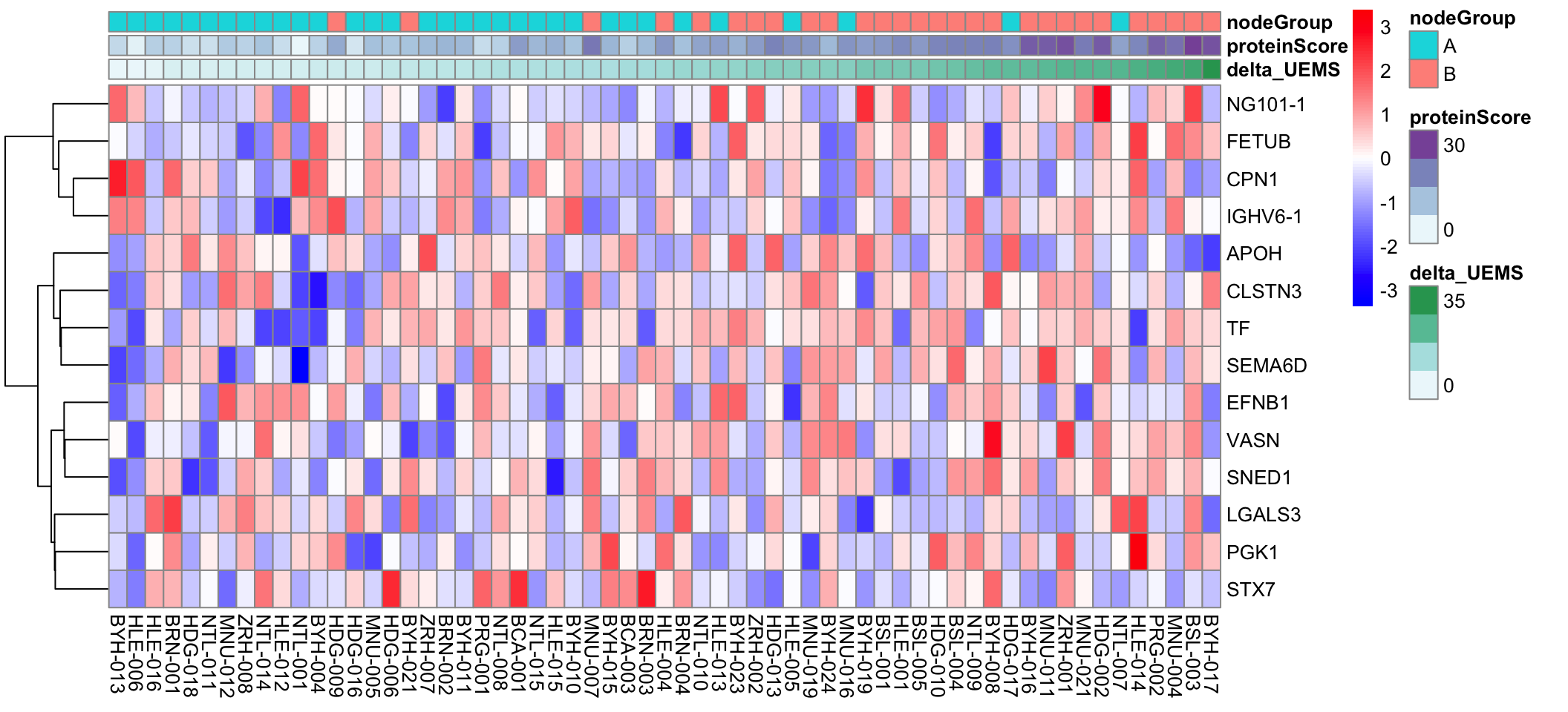

Visualize the 10 features from the V3 dataset

seleFeature <- filter(rndRes, set == "V3") %>%
    slice_max(importance, n=10) %>% pull(feature)

#predict the score
X <- t(allTrainData[["V3"]]$X)[,seleFeature]
y <- allTrainData[["V3"]]$y
seleModel <- glmnet(X, y, lambda =0)
y.pred <- predict(seleModel, newx = X)[,1]
scoreList[["V3_10"]] <- y.pred


plotMat <- allTrainData$V3$X[seleFeature,]
annoCol <- data.frame(row.names = colnames(plotMat), delta_UEMS = allTrainData$V3$y, 
                      proteinScore = y.pred,
                      nodeGroup = protV3[,colnames(plotMat)]$nodeGroup)
annoCol <- annoCol[order(annoCol$delta_UEMS),,drop=FALSE]
plotMat <- plotMat[,rownames(annoCol)]
pheatmap::pheatmap(plotMat, annotation_col = annoCol, cluster_rows = TRUE, cluster_cols = FALSE, scale = "row",
                   clustering_method = "ward.D2",
                   color = colorRampPalette(c("blue", "white", "red"))(100))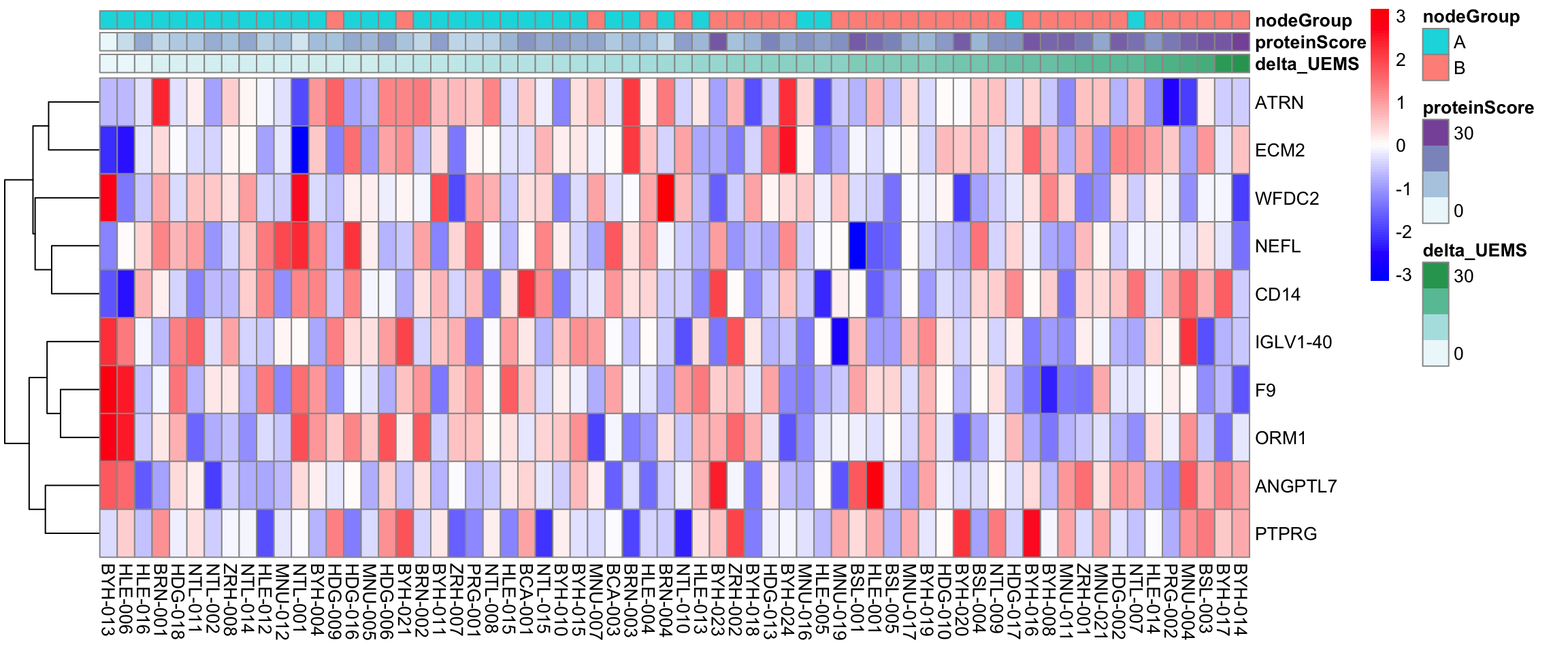

Test the score performance in multi-variate models including other clinical paramters

Prepare a table for other clinical parameters

Those parameter will be included: Age, Sex, UEMS at Visit 3, AIS, random node group (A or B)

patAnno <- colData(seProt) %>% as_tibble() %>% filter(Treatment =="1")

scaleCol <- function(x){
  return((x-mean(x,na.rm=TRUE))/sd(x, na.rm=TRUE))
}

clinicTab <- arrange(patAnno, Visit) %>% distinct(PSN,.keep_all = TRUE) %>%
  select(PSN, SEX, AGE, AIS, nodeGroup, delta_UEMS) %>%
  mutate_if(is.numeric, scaleCol)
  

uemsTab <- distinct(patAnno, PSN, Visit, UEMS) %>%
  mutate(Visit = paste0("UEMS_V",Visit)) %>%
  pivot_wider(names_from = Visit, values_from = UEMS) %>%
  #mutate(UEMS_diff38 = UEMS_V8/UEMS_V3) %>%
  select(PSN, UEMS_V3)

clinicTab <- left_join(clinicTab, uemsTab, by = "PSN") %>%
  mutate_if(is.character, as.factor) %>%
  mutate(PSN = as.character(PSN))

Test performance of model with only clinical parameter, protein score and clinical paremeter + protein score

With the combine_15 protein score

Prediction accuracy

allModels <- list()
allModels[["combine"]] <- clinicTab %>% mutate(proteinScore = scoreList$combine_15[PSN]) %>%
  column_to_rownames("PSN") %>% data.frame()
allModels[["onlyClinic"]] <- clinicTab %>% 
  column_to_rownames("PSN") %>% data.frame()
allModels[["onlyProtein"]] <- allModels$combine[,c("delta_UEMS","proteinScore")]

plotResTab <- lapply(names(allModels), function(nn) {
  eachModel <- allModels[[nn]]
  res <- summary(lm(delta_UEMS~. ,eachModel))
  tibble(model = nn, R2 = res$adj.r.squared)
}) %>% bind_rows()
ggplot(plotResTab, aes(x=model, y=R2, fill = model)) +
  geom_bar(stat = "identity") +
  coord_flip() +
  ylim(0,1) +
  theme_bw() + theme(legend.position = "none") +
  ylab("Variance explained")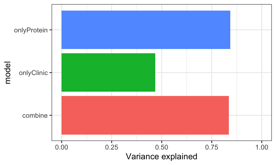

The higher the variance explained, the better the models are

Forest plot for feature importance and significance

res <- summary(lm(delta_UEMS~. ,allModels$combine))
plotForest(res)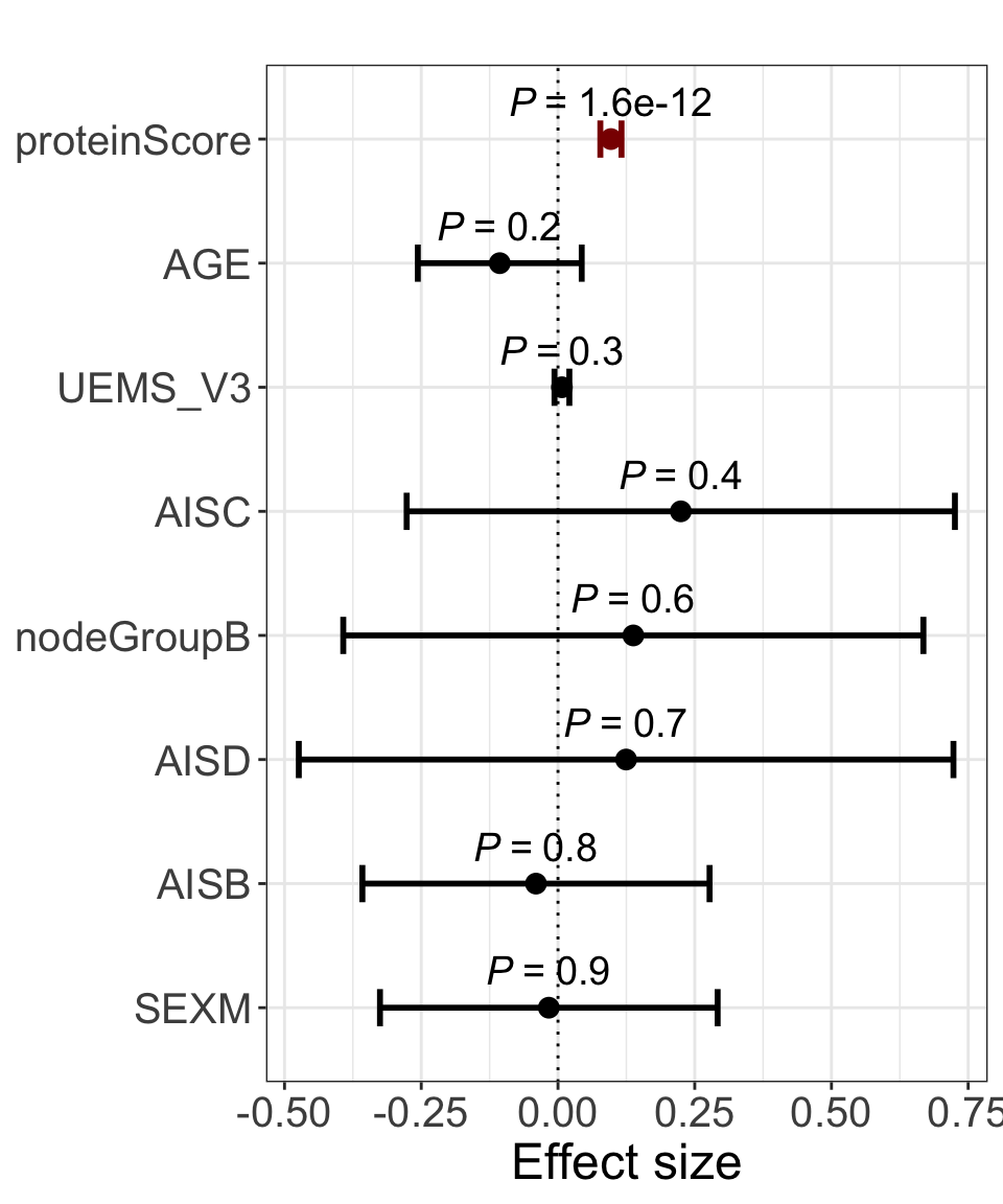

With the V8_14 score

Prediction accuracy

allModels <- list()
allModels[["combine"]] <- clinicTab %>% mutate(proteinScore = scoreList$V8_14[PSN]) %>%
  column_to_rownames("PSN") %>% data.frame()
allModels[["onlyClinic"]] <- clinicTab %>% 
  column_to_rownames("PSN") %>% data.frame()
allModels[["onlyProtein"]] <- allModels$combine[,c("delta_UEMS","proteinScore")]

plotResTab <- lapply(names(allModels), function(nn) {
  eachModel <- allModels[[nn]]
  res <- summary(lm(delta_UEMS~. ,eachModel))
  tibble(model = nn, R2 = res$adj.r.squared)
}) %>% bind_rows()
ggplot(plotResTab, aes(x=model, y=R2, fill = model)) +
  geom_bar(stat = "identity") +
  coord_flip() +
  theme_bw() + theme(legend.position = "none") +
  ylim(0,1)

Forest plot for feature importance and significance

res <- summary(lm(delta_UEMS~. ,allModels$combine))
plotForest(res)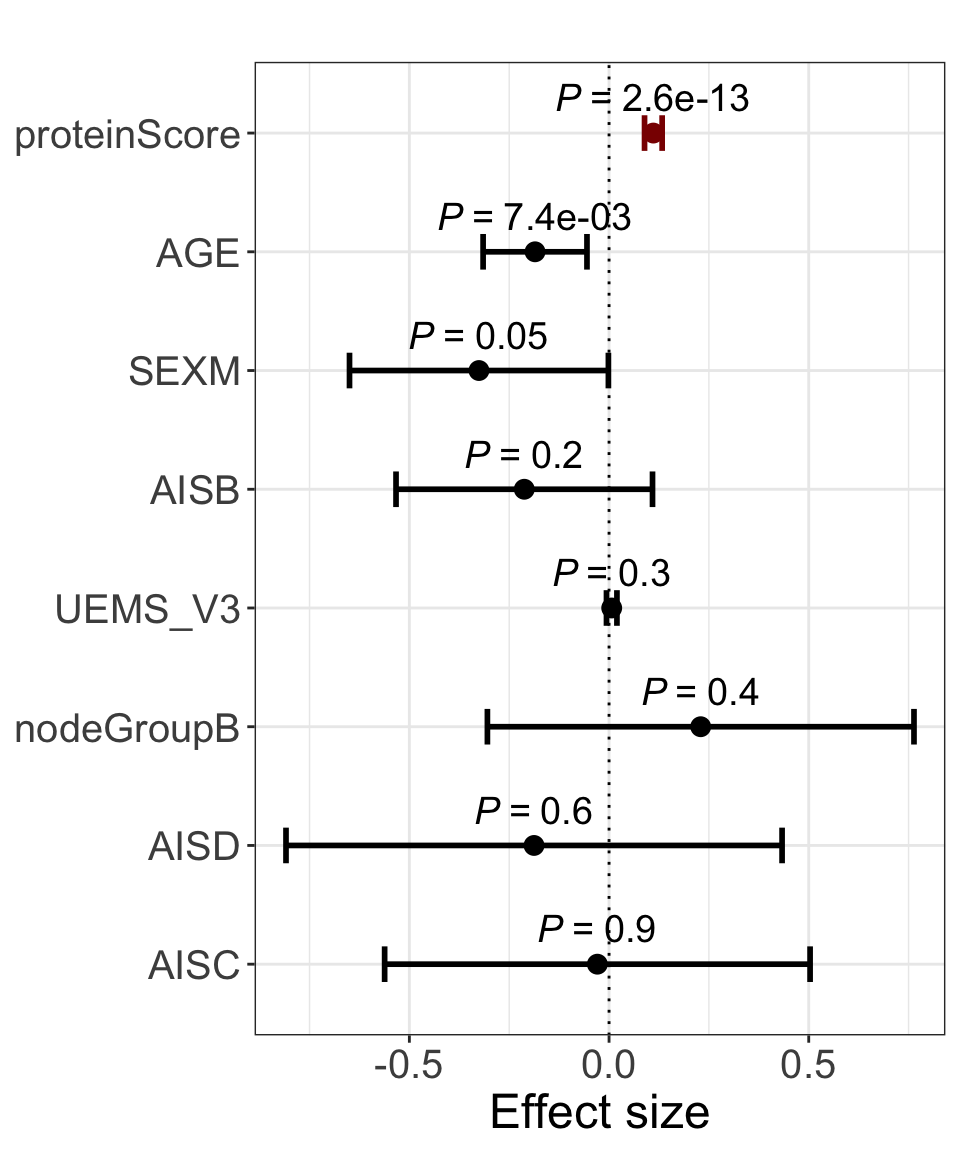

Forest plot for only clinical variables

res <- summary(lm(delta_UEMS~. ,allModels$onlyClinic))
plotForest(res)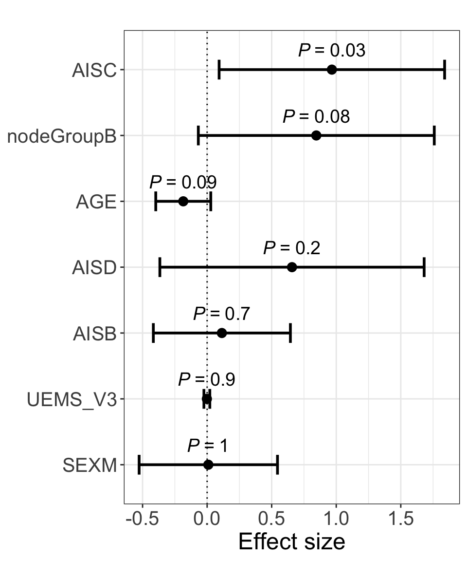

With the V3_10 score

Prediction accuracy

allModels <- list()
allModels[["combine"]] <- clinicTab %>% mutate(proteinScore = scoreList$V3_10[PSN]) %>%
  column_to_rownames("PSN") %>% data.frame()
allModels[["onlyClinic"]] <- clinicTab %>% 
  column_to_rownames("PSN") %>% data.frame()
allModels[["onlyProtein"]] <- allModels$combine[,c("delta_UEMS","proteinScore")]

plotResTab <- lapply(names(allModels), function(nn) {
  eachModel <- allModels[[nn]]
  res <- summary(lm(delta_UEMS~. ,eachModel))
  tibble(model = nn, R2 = res$adj.r.squared)
}) %>% bind_rows()
ggplot(plotResTab, aes(x=model, y=R2, fill = model)) +
  geom_bar(stat = "identity") +
  coord_flip() +
  theme_bw() + theme(legend.position = "none") +
  ylim(0,1)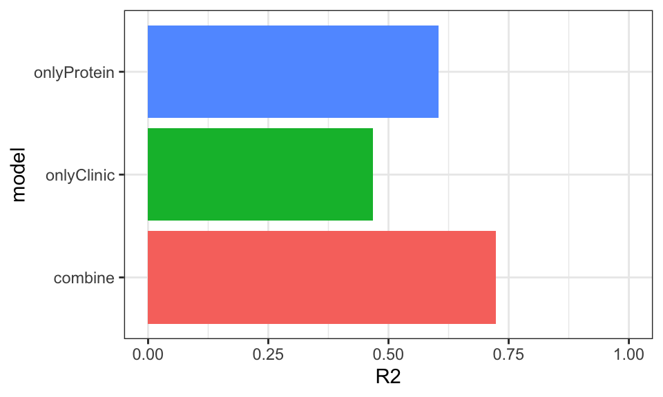

Forest plot for feature importance and significance

res <- summary(lm(delta_UEMS~. ,allModels$combine))
plotForest(res)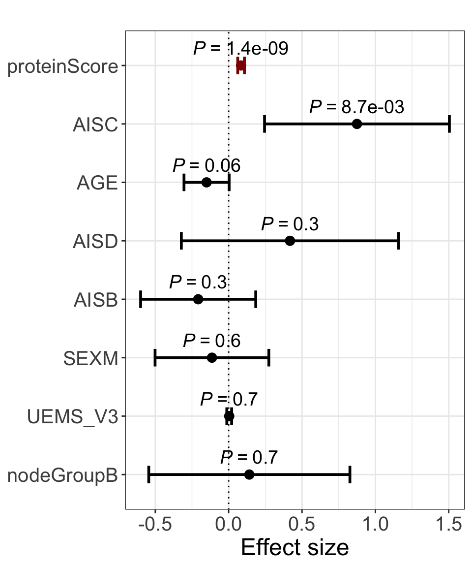

Session information

sessionInfo()

R version 4.2.0 (2022-04-22)
Platform: x86_64-apple-darwin17.0 (64-bit)
Running under: macOS Big Sur/Monterey 10.16

Matrix products: default
BLAS:   /Library/Frameworks/R.framework/Versions/4.2/Resources/lib/libRblas.0.dylib
LAPACK: /Library/Frameworks/R.framework/Versions/4.2/Resources/lib/libRlapack.dylib

locale:
[1] en_US.UTF-8/en_US.UTF-8/en_US.UTF-8/C/en_US.UTF-8/en_US.UTF-8

attached base packages:
[1] stats4    stats     graphics  grDevices utils     datasets  methods  
[8] base     

other attached packages:
 [1] forcats_0.5.1               stringr_1.4.1              
 [3] dplyr_1.1.4.9000            purrr_0.3.4                
 [5] readr_2.1.2                 tidyr_1.2.0                
 [7] tibble_3.2.1                ggplot2_3.4.1              
 [9] tidyverse_1.3.2             glmnet_4.1-4               
[11] Matrix_1.5-4                sva_3.44.0                 
[13] BiocParallel_1.30.3         genefilter_1.78.0          
[15] mgcv_1.8-40                 nlme_3.1-158               
[17] limma_3.52.2                SummarizedExperiment_1.26.1
[19] Biobase_2.56.0              GenomicRanges_1.48.0       
[21] GenomeInfoDb_1.32.2         IRanges_2.30.0             
[23] S4Vectors_0.34.0            BiocGenerics_0.42.0        
[25] MatrixGenerics_1.8.1        matrixStats_0.62.0         

loaded via a namespace (and not attached):
  [1] utf8_1.2.4             shinydashboard_0.7.2   tidyselect_1.2.1      
  [4] RSQLite_2.2.15         AnnotationDbi_1.58.0   htmlwidgets_1.5.4     
  [7] grid_4.2.0             maxstat_0.7-25         munsell_0.5.0         
 [10] codetools_0.2-18       DT_0.23                withr_3.0.0           
 [13] colorspace_2.0-3       highr_0.9              knitr_1.39            
 [16] rstudioapi_0.13        ggsignif_0.6.3         labeling_0.4.2        
 [19] git2r_0.30.1           slam_0.1-50            GenomeInfoDbData_1.2.8
 [22] KMsurv_0.1-5           bit64_4.0.5            farver_2.1.1          
 [25] pheatmap_1.0.12        rprojroot_2.0.3        vctrs_0.6.5           
 [28] generics_0.1.3         TH.data_1.1-1          xfun_0.31             
 [31] sets_1.0-21            R6_2.5.1               locfit_1.5-9.6        
 [34] bitops_1.0-7           cachem_1.0.6           fgsea_1.22.0          
 [37] DelayedArray_0.22.0    assertthat_0.2.1       promises_1.2.0.1      
 [40] scales_1.2.0           multcomp_1.4-19        googlesheets4_1.0.0   
 [43] gtable_0.3.0           sandwich_3.0-2         workflowr_1.7.0       
 [46] rlang_1.1.3            splines_4.2.0          rstatix_0.7.0         
 [49] gargle_1.2.0           broom_1.0.0            BiocManager_1.30.18   
 [52] yaml_2.3.5             abind_1.4-5            modelr_0.1.8          
 [55] backports_1.4.1        httpuv_1.6.6           tools_4.2.0           
 [58] relations_0.6-12       ellipsis_0.3.2         gplots_3.1.3          
 [61] RColorBrewer_1.1-3     jquerylib_0.1.4        Rcpp_1.0.9            
 [64] visNetwork_2.1.0       zlibbioc_1.42.0        RCurl_1.98-1.7        
 [67] ggpubr_0.4.0           cowplot_1.1.1          zoo_1.8-10            
 [70] haven_2.5.0            cluster_2.1.3          exactRankTests_0.8-35 
 [73] fs_1.5.2               magrittr_2.0.3         data.table_1.14.8     
 [76] reprex_2.0.1           survminer_0.4.9        googledrive_2.0.0     
 [79] mvtnorm_1.1-3          hms_1.1.1              shinyjs_2.1.0         
 [82] mime_0.12              evaluate_0.15          xtable_1.8-4          
 [85] XML_3.99-0.10          readxl_1.4.0           gridExtra_2.3         
 [88] shape_1.4.6            compiler_4.2.0         KernSmooth_2.23-20    
 [91] crayon_1.5.2           htmltools_0.5.4        later_1.3.0           
 [94] tzdb_0.3.0             lubridate_1.8.0        DBI_1.1.3             
 [97] dbplyr_2.2.1           MASS_7.3-58            jyluMisc_0.1.5        
[100] BiocStyle_2.24.0       car_3.1-0              cli_3.6.2             
[103] marray_1.74.0          parallel_4.2.0         igraph_1.3.4          
[106] pkgconfig_2.0.3        km.ci_0.5-6            piano_2.12.0          
[109] xml2_1.3.3             foreach_1.5.2          annotate_1.74.0       
[112] bslib_0.4.1            XVector_0.36.0         drc_3.0-1             
[115] rvest_1.0.2            digest_0.6.30          Biostrings_2.64.0     
[118] rmarkdown_2.14         cellranger_1.1.0       fastmatch_1.1-3       
[121] survMisc_0.5.6         edgeR_3.38.1           shiny_1.7.4           
[124] gtools_3.9.3           lifecycle_1.0.4        jsonlite_1.8.3        
[127] carData_3.0-5          fansi_1.0.6            pillar_1.9.0          
[130] lattice_0.20-45        KEGGREST_1.36.3        fastmap_1.1.0         
[133] httr_1.4.3             plotrix_3.8-2          survival_3.4-0        
[136] glue_1.7.0             png_0.1-7              iterators_1.0.14      
[139] bit_4.0.4              stringi_1.7.8          sass_0.4.2            
[142] blob_1.2.3             caTools_1.18.2         memoise_2.0.1