Data preprocessing and QA
Junyan Lu
Last updated: 2024-04-24
Checks: 5 1
Knit directory:
SpinalCord_proteomics/analysis/
This reproducible R Markdown analysis was created with workflowr (version 1.7.0). The Checks tab describes the reproducibility checks that were applied when the results were created. The Past versions tab lists the development history.
Great job! The global environment was empty. Objects defined in the global environment can affect the analysis in your R Markdown file in unknown ways. For reproduciblity it’s best to always run the code in an empty environment.
The command set.seed(20221110) was run prior to running
the code in the R Markdown file. Setting a seed ensures that any results
that rely on randomness, e.g. subsampling or permutations, are
reproducible.
Great job! Recording the operating system, R version, and package versions is critical for reproducibility.
Nice! There were no cached chunks for this analysis, so you can be confident that you successfully produced the results during this run.
Great job! Using relative paths to the files within your workflowr project makes it easier to run your code on other machines.
Tracking code development and connecting the code version to the
results is critical for reproducibility. To start using Git, open the
Terminal and type git init in your project directory.
This project is not being versioned with Git. To obtain the full
reproducibility benefits of using workflowr, please see
?wflow_start.
Data preprocessing
Read in proteomics data
protTab <- read_csv("../data/SPECTRO_MS_DATA.csv") %>%
    dplyr::select(-`T: PG.Organisms`) %>%
    dplyr::rename(uniprotID = "T: PG.ProteinAccessions",
                  symbol = "T: PG.Genes",
                  description = "T: PG.ProteinDescriptions") %>%
    pivot_longer(-c(uniprotID, symbol, description),
                 names_to = "sampleID",
                 values_to = "count")
Read annotation table
sampleTab <- tibble(sampleID = unique(protTab$sampleID))

#clinical information
clinicTab <- read_csv("../data/SPECTRO_CLINICAL_DATA.csv")
sampleTab <- left_join(sampleTab, clinicTab, by = c(sampleID = "Column-Header in quant tabel")) %>%
    dplyr::rename(boID = `BO-ID`, rawFileInternal = `raw file-intern`, Visit = Vistit) %>%
    mutate(Treatment = ifelse(is.na(Treatment),"control",Treatment))

#treatment information
treatTab <- read_csv("../data/long_ISNT.csv") %>%
    mutate(Visit = case_when(VISITNUM == 2 ~ 3,
                             VISITNUM == 9 ~ 8,
                             VISITNUM == 10 ~ 10))

sampleTab <- left_join(sampleTab, treatTab, by = c(PSN =  "USUBJID", Visit = "Visit"))
#may not be useful for now, leave it aside.
The CSF-sampling visits were: V3 (right before first Dosing) – corresponding clinical visit V2 (baseline) V8 (last dosing at around 1 month) – corresponding clinical visit V9 (1month) V10 (3 months) – corresponding clinical visit V10 (3 months)
Combine the proteomic data and sample info into a SE object
comTab <- left_join(protTab, sampleTab, by = "sampleID")
seProt <- jyluMisc::tidyToSum(comTab, rowID = "uniprotID", colID = "sampleID", values = "count",
                              annoRow = c("uniprotID","symbol","description"),
                              annoCol = colnames(sampleTab))
Reformat for DEP
rowData(seProt)$ID <- rowData(seProt)$uniprotID
rowData(seProt)$name <- rowData(seProt)$symbol
Data dimension
dim(seProt)[1] 473 333Quality check
Examin the data distrubution
countMat <- assay(seProt)Boxplot including all proteins
boxplot(countMat)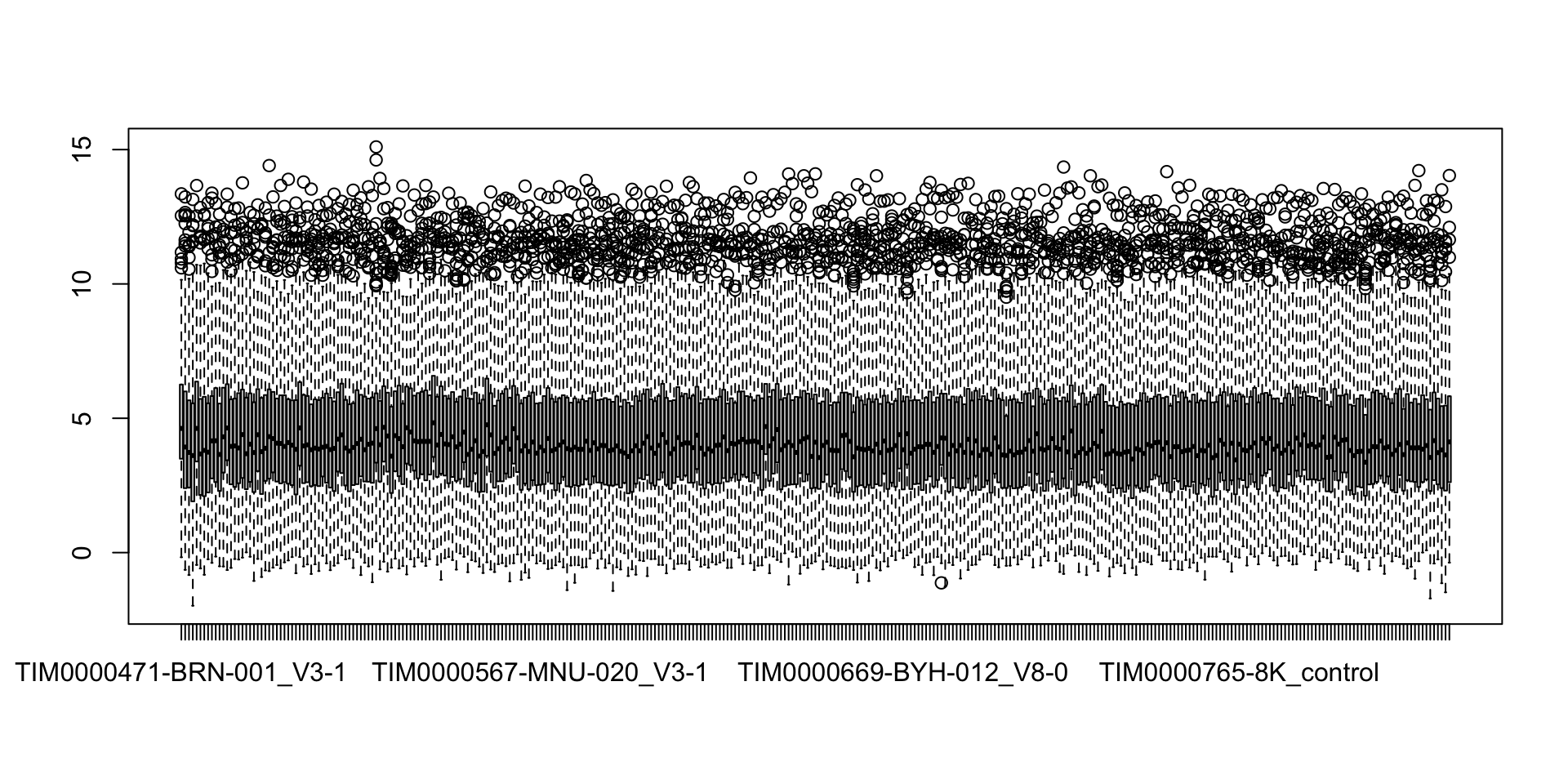 Seems already transformed. Not sure if already normalized. (What
transformation function was used?)
Seems already transformed. Not sure if already normalized. (What
transformation function was used?)
Boxplot of proteins with less than 50% missingness
countMat.sub <- countMat[rowSums(is.na(countMat))/ncol(countMat) < 0.5,]
boxplot(countMat.sub)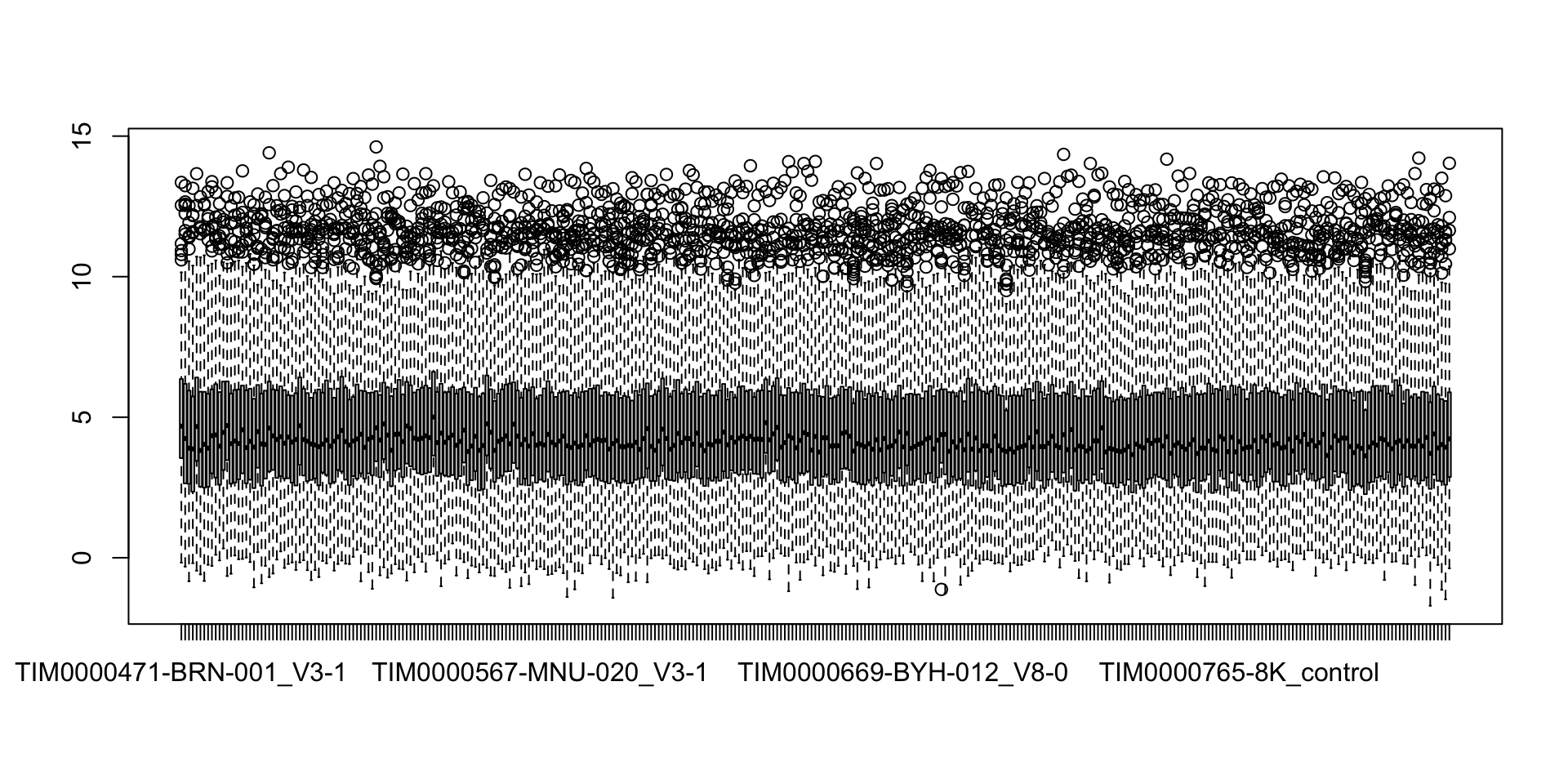
Missing value per sample
plotTab <- tibble(sample = seProt$sampleID,
                  perNA = colSums(is.na(countMat))/nrow(countMat),
                  total = colSums(countMat, na.rm=TRUE),
                  medVal = colMedians(countMat, na.rm=TRUE))

plotTab <- plotTab %>% arrange(desc(perNA)) %>%
    mutate(sample  = factor(sample, levels = sample))

ggplot(plotTab, aes(x=sample, y=1-perNA)) +
    geom_bar(stat = "identity") +
    ylab("completeness") +
theme(axis.text.x = element_text(angle = 90, hjust = 1, vjust=0)) 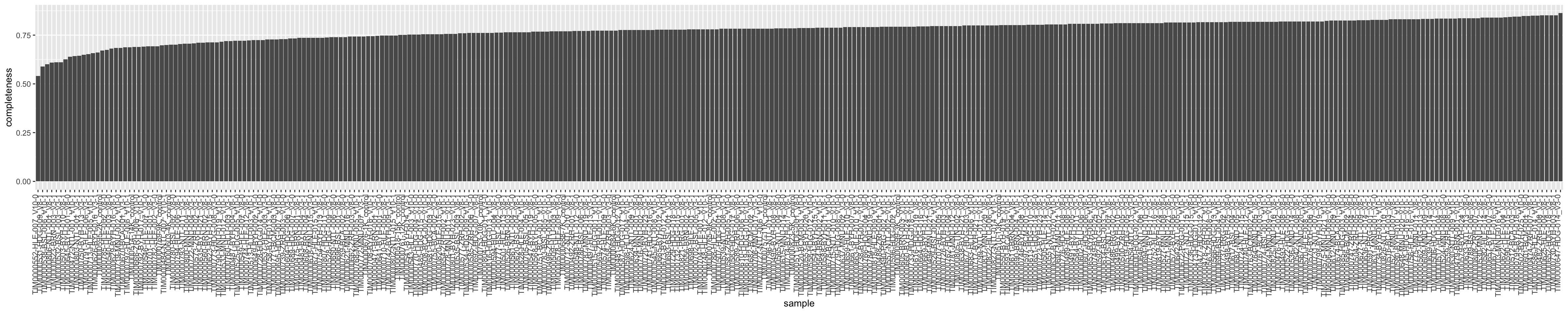
totalQuantTab <- plotTabTotal intensity
plotTab <- plotTab %>% arrange(total) %>%
    mutate(sample  = factor(sample, levels = sample))

ggplot(plotTab, aes(x=sample, y=total)) +
    geom_bar(stat = "identity") +
    ylab("total intensity") +
theme(axis.text.x = element_text(angle = 90, hjust = 1, vjust=0)) 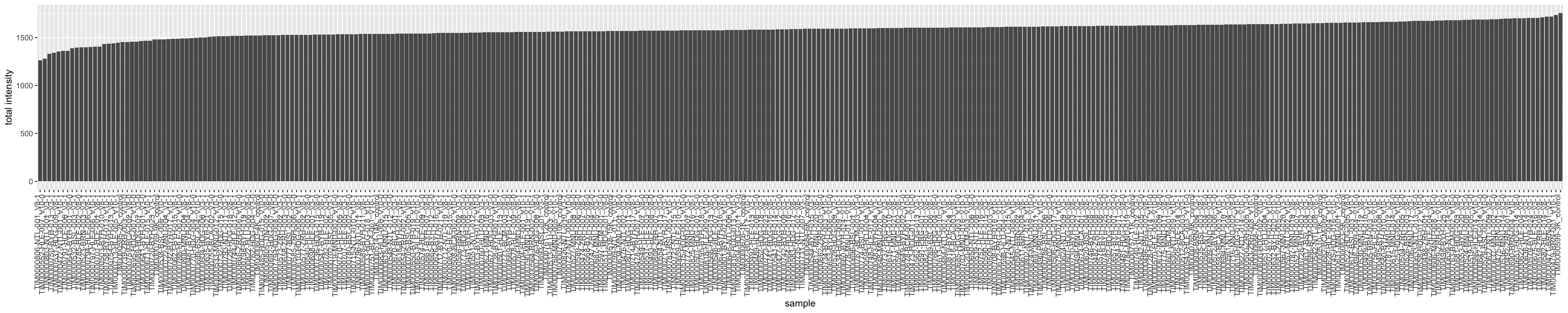
Median Intensity
plotTab <- plotTab %>% arrange(medVal) %>%
    mutate(sample  = factor(sample, levels = sample))

ggplot(plotTab, aes(x=sample, y=medVal)) +
    geom_bar(stat = "identity") +
    ylab("median intensity") +
theme(axis.text.x = element_text(angle = 90, hjust = 1, vjust=0)) 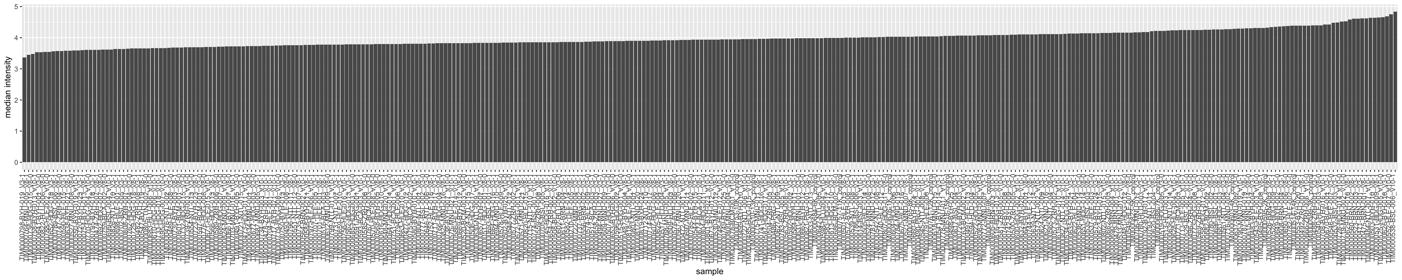
Boxplots showing the distribution
boxTab <- assay(seProt) %>% as_tibble(rownames = "id") %>%
  pivot_longer(-id) %>%
  mutate(perNA = plotTab[match(name, plotTab$sample),]$perNA) %>%
  mutate(name = factor(name, levels = arrange(plotTab, desc(medVal))$sample))

ggplot(boxTab, aes(x=name, y=value)) +
  geom_boxplot(aes(fill = perNA)) +
  theme(axis.text.x = element_text(angle = 90, hjust = 1, vjust = 0.5))
#### Pairwise correlation of the metrics
Completeness versus total
ggplot(plotTab, aes(x=1-perNA, y=total)) +
  geom_point()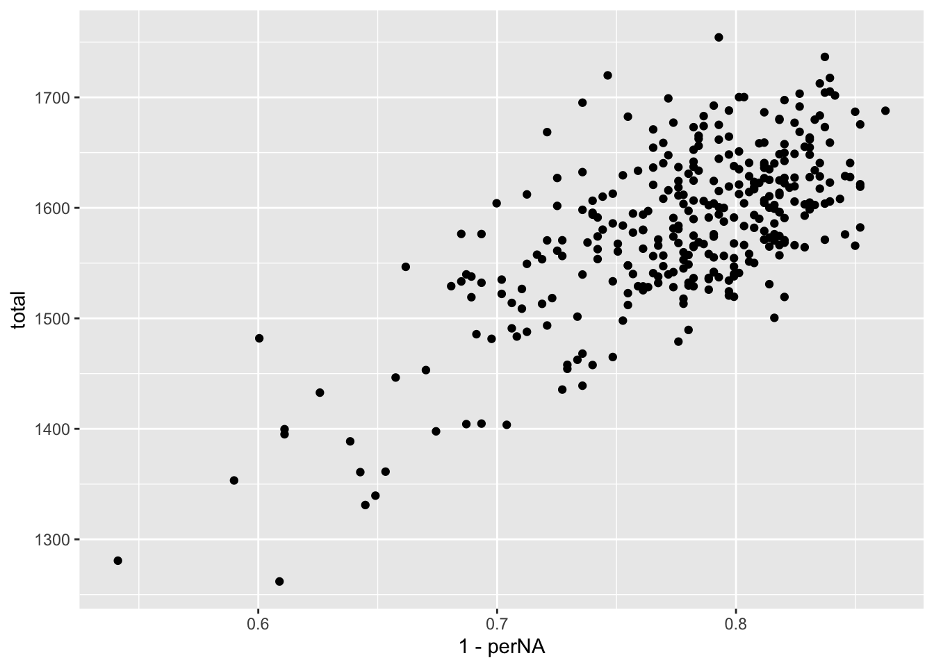
median versus total
ggplot(plotTab, aes(x=medVal, y=total)) +
  geom_point()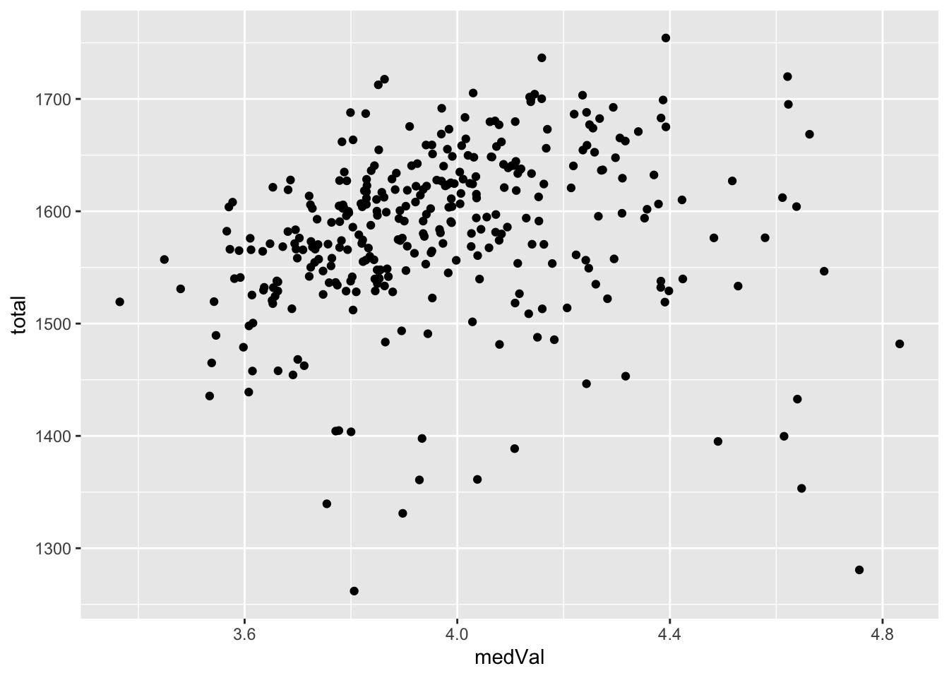
median versus completeness
ggplot(plotTab, aes(x=medVal, y=1-perNA)) +
  geom_point()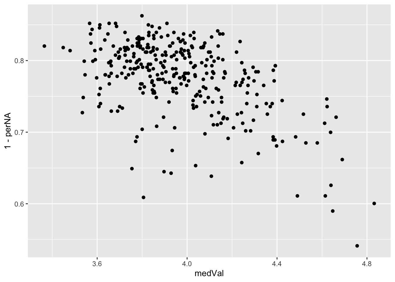
Pairwise-MA plot
Function for MA plot give a sample list
plotMA <- function(sampleList, protData, sampleList2 = NULL, logTransform=FALSE) {
  if (is.null(sampleList2)) {
    allCombo <- combn(sampleList, 2)
  } else {
    n1 <- length(sampleList)
    n2 <- length(sampleList2)
    allCombo <- matrix(rep(NA, n1*n2*2), nrow=2, ncol=n1*n2)
    n <- 1
    for (each1 in sampleList) {
      for (each2 in sampleList2) {
        allCombo[,n] <- c(each1, each2)
        n <- n + 1
      }
    }
  }
  if (logTransform) {
    assay(protData) <- log2(assay(protData))
  }
  pList <- apply(allCombo, 2, function(x) {
    exp1 <- assay(protData)[,x[1]]
    exp2 <- assay(protData)[,x[2]]
    eachTab <- tibble(M = exp1-exp2, A = (exp1+exp2)/2)
    ggplot(eachTab, aes(x=A,y=M)) +
      geom_point(shape =1) +
      geom_smooth(se=FALSE, color = "red") +
      ggtitle(sprintf("%s ~ %s",x[1],x[2])) +
      theme(plot.title = element_text(size=8))
  })
  cowplot::plot_grid(plotlist = pList, ncol=2)
}
Samples with most missing values
sampleList <- arrange(plotTab, total)$sample[1:5]
plotMA(sampleList, seProt, logTransform = FALSE)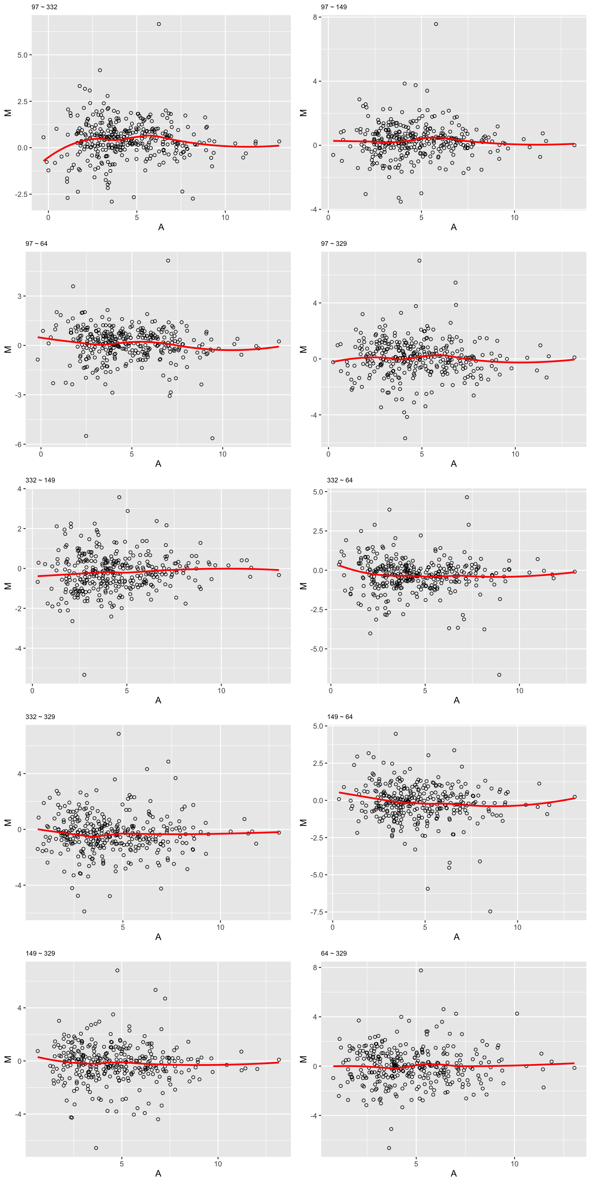
Samples with least missing values
dsampleList <- arrange(plotTab, perNA)$sample[1:5]
plotMA(sampleList, seProt, logTransform = FALSE)
Between samples of most and list missing values
sampleList1 <- arrange(plotTab, perNA)$sample[1:4]
sampleList2 <- arrange(plotTab, desc(perNA))$sample[1:4]
plotMA(sampleList1, seProt, sampleList2 = sampleList2, logTransform = TRUE)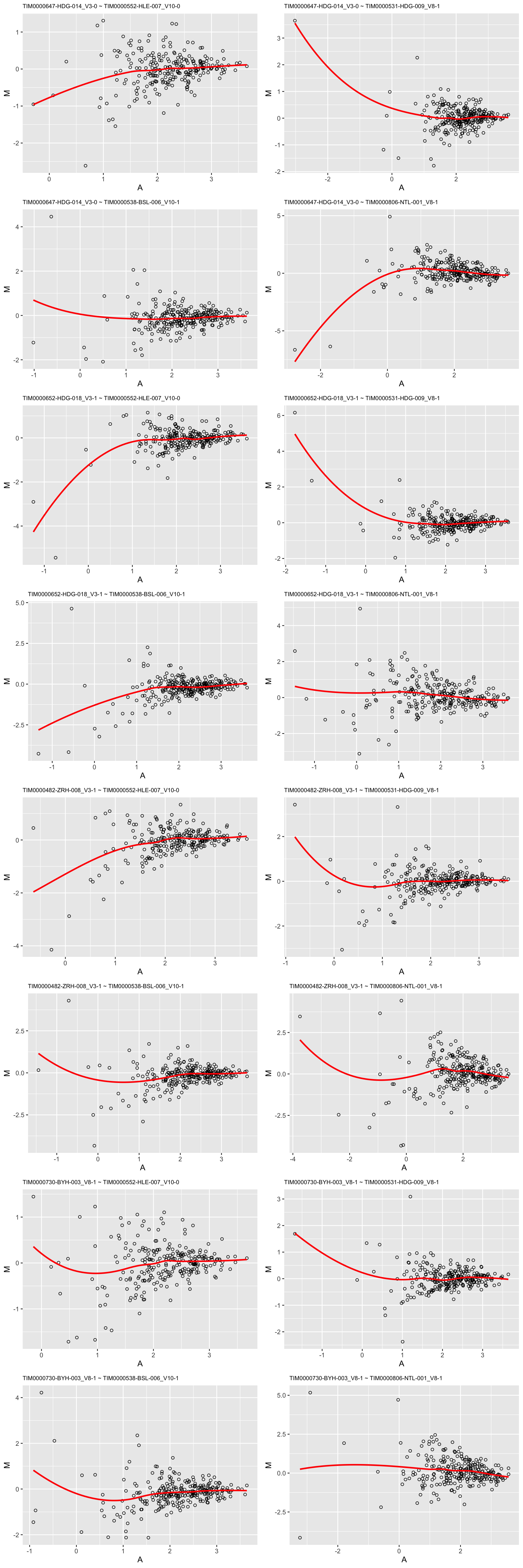
Variance versus mean
vsn::meanSdPlot(countMat)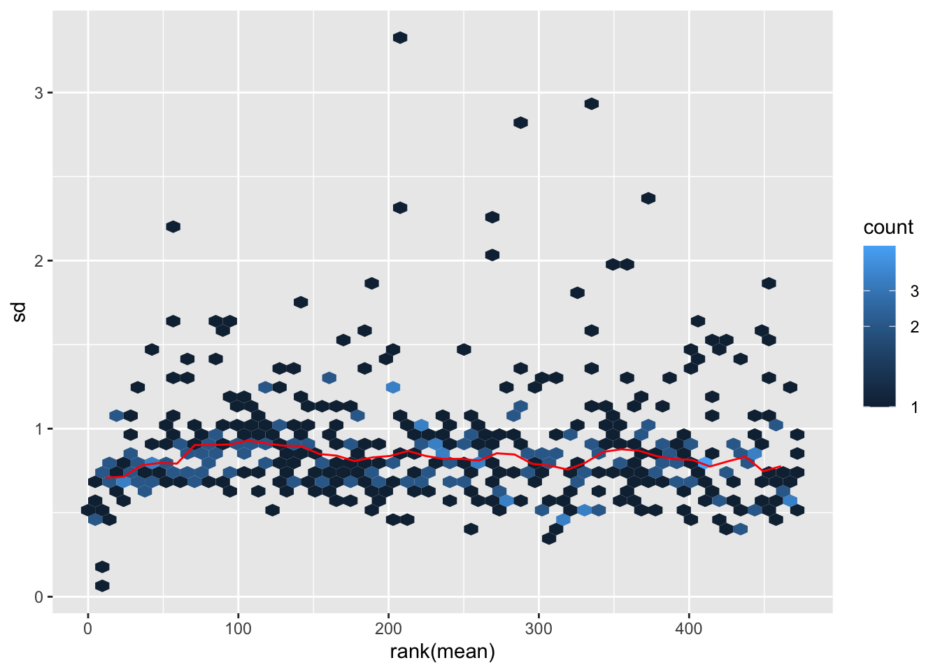
Missing value pattern
plotTab <- tibble(meanVal = rowMeans(countMat, na.rm=TRUE),
                  dropOut = rowMeans(is.na(countMat)))
ggplot(plotTab, aes(x=meanVal, y=dropOut)) +
    geom_point()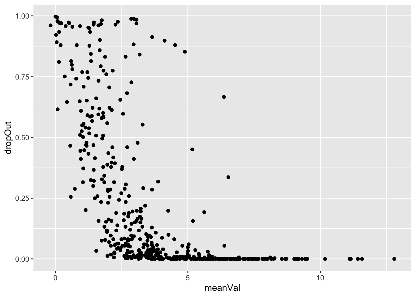
Missing value pattern as heatmap
DEP::plot_missval(seProt)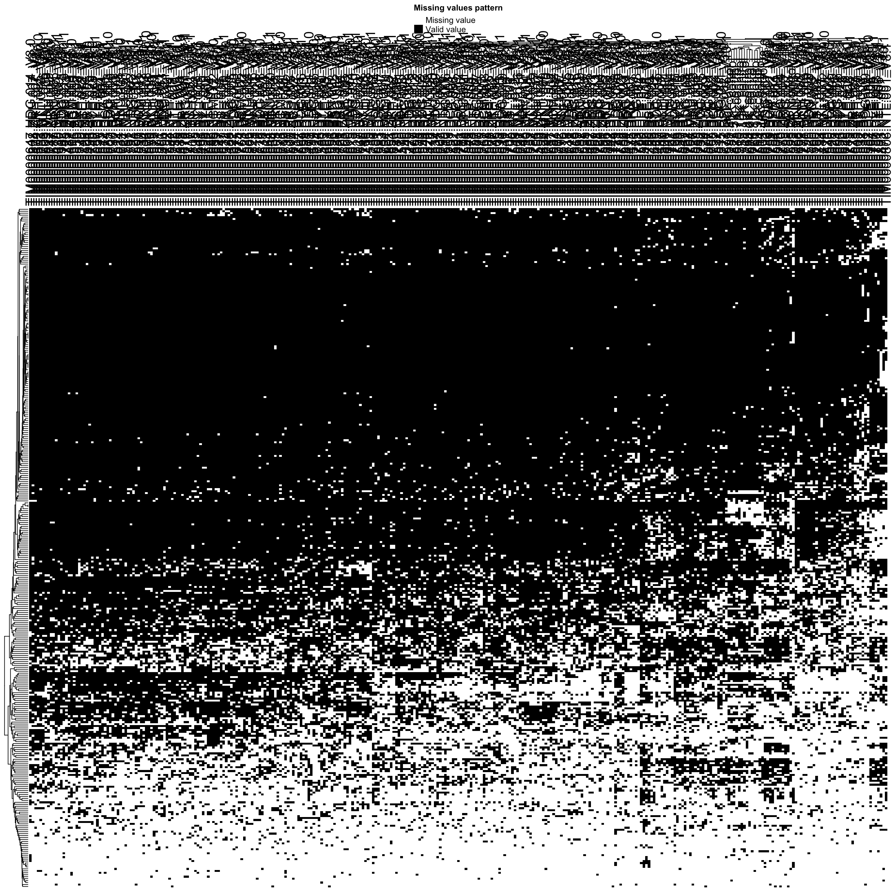
Missing value cut-off versus number of remaining proteins
missPer <- rowSums(is.na(countMat))/ncol(countMat)
sumTab <- lapply(seq(0,1,by = 0.01), function(x) tibble(cut = x, freq = sum(missPer < x)/length(missPer))) %>% bind_rows()
ggplot(sumTab, aes(x=cut, y=freq)) + geom_line() + xlab("Missing value cut-off") + ylab("Percent remaining") +
  scale_x_continuous(breaks = seq(0,1, 0.1))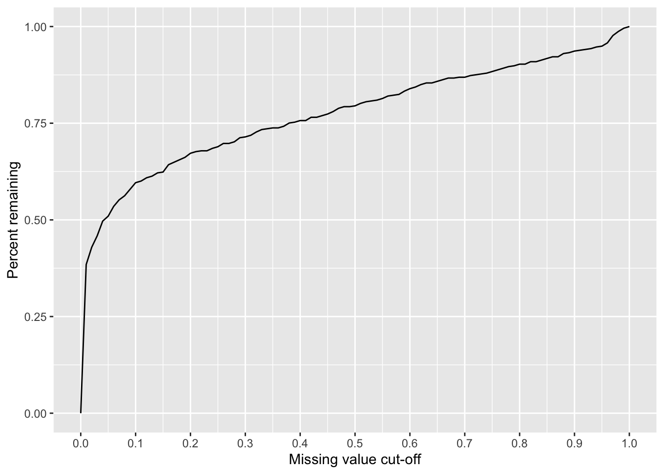
Remove proteins with more than 50% missing values
seProt_raw <- seProt
cut=0.5
seProt <- seProt[rowSums(is.na(assay(seProt)))/ncol(seProt) <= cut,]
dim(seProt)
[1] 376 333#assayNames(protData_filter) <- "norm"Impute missing values using bpca
Using BPCA imputation
seImp <- seProt
seImp <- DEP::impute(seImp, fun = "bpca")
assays(seProt)[["imputed"]] <- assay(seImp)
Save processed data
save(seProt, seProt_raw, file = "../output/seProt.RData")Exploratory data analysis
Load processed data
load("../output/seProt.RData")PCA
exprMat <- assays(seProt)[["imputed"]]

smpAnno <- colData(seProt) %>% as_tibble()

pcRes <- prcomp(t(exprMat), scale. = FALSE, center = TRUE)

pcTab <- pcRes$x[,1:20] %>%
    as_tibble(rownames = "sampleID")

plotTab <- pcTab %>%
    left_join(smpAnno)

varExp <- pcRes$sdev^2/sum(pcRes$sdev^2) * 100
Test associations between PCA and metadata
metaTab <- smpAnno %>%
  select(sampleID, PSN, Visit, Treatment, Node, delta_UEMS, UEMS, SEX, AGE, AIS) %>%
    left_join(totalQuantTab, by =c(sampleID = "sample"))

resTab <- jyluMisc::testAssociation(pcTab, metaTab, joinID = "sampleID", plot = TRUE, ifFdr = TRUE, pCut = 0.05)
head(resTab$resTab)
var1 var2 p p.adj
1 PC1 total 3.813979e-47 9.153551e-45
2 PC4 Treatment 2.515533e-32 3.018640e-30
3 PC5 Visit 5.652751e-31 4.522201e-29
4 PC1 PSN 1.005890e-30 6.035337e-29
5 PC4 PSN 2.226015e-27 1.068487e-25
6 PC3 medVal 2.982878e-24 1.193151e-22resTab$plot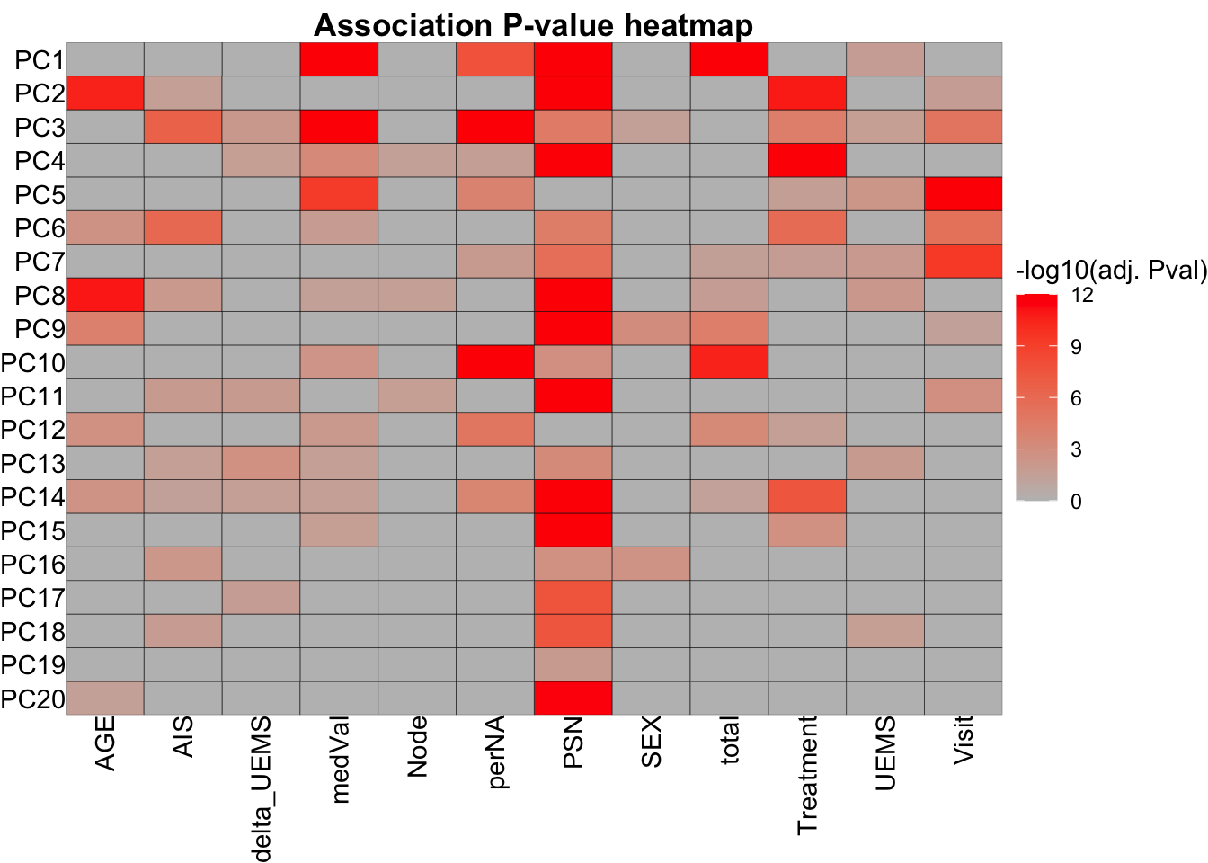
Plots
PC1 versus PC2
ggplot(plotTab, aes(x=PC1, y=PC2, shape = factor(Treatment), color= delta_UEMS)) +
    geom_point() +
    xlab(sprintf("PC1 (%1.2f%%)",varExp[1])) +
    ylab(sprintf("PC2 (%1.2f%%)",varExp[2])) +
    theme_bw()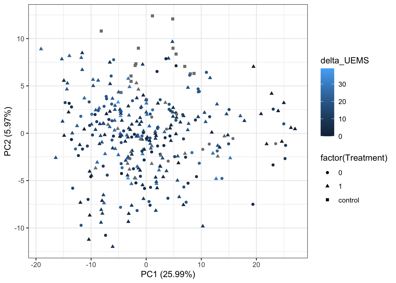
PC4 versus PC5
ggplot(plotTab, aes(x=PC4, y=PC5, shape = factor(Treatment), color= Visit)) +
    geom_point() +
    xlab(sprintf("PC4 (%1.2f%%)",varExp[4])) +
    ylab(sprintf("PC5 (%1.2f%%)",varExp[5])) +
    theme_bw()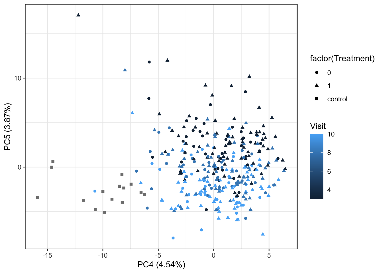
PCA after adjustment for patient specific effect
Since patient heterogneity dominates the variance, we can try to remove it first
exprMat <- assays(seProt)[["imputed"]]
exprMat.combat <- sva::ComBat(exprMat, batch = seProt$PSN)
assays(seProt)[["combat"]] <- exprMat.combat
exprMat <- assays(seProt)[["combat"]]
pcRes <- prcomp(t(exprMat), scale. = FALSE, center = TRUE)
pcTab <- pcRes$x[,1:20] %>%
as_tibble(rownames = "sampleID")
plotTab <- pcTab %>%
left_join(smpAnno)
varExp <- pcRes$sdev^2/sum(pcRes$sdev^2) * 100Test associations between PCA and metadata
resTab <- jyluMisc::testAssociation(pcTab, metaTab, joinID = "sampleID", plot = TRUE, ifFdr = TRUE, pCut = 0.05)
head(resTab$resTab)
var1 var2 p p.adj
1 PC2 Visit 9.070501e-36 2.176920e-33
2 PC3 Visit 1.631405e-24 1.957686e-22
3 PC1 total 4.105926e-17 3.284741e-15
4 PC3 medVal 8.253500e-17 4.952100e-15
5 PC1 medVal 1.620271e-14 7.777303e-13
6 PC3 perNA 1.536859e-12 6.147438e-11resTab$plot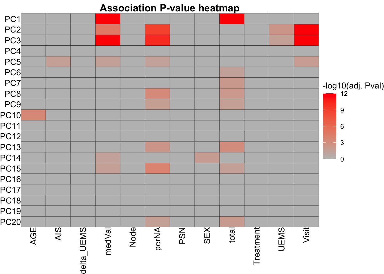
Plots
PC1 versus PC2
ggplot(plotTab, aes(x=PC1, y=PC2, shape = factor(Treatment), color= factor(Visit))) +
    geom_point() +
    xlab(sprintf("PC1 (%1.2f%%)",varExp[1])) +
    ylab(sprintf("PC2 (%1.2f%%)",varExp[2])) +
    theme_bw()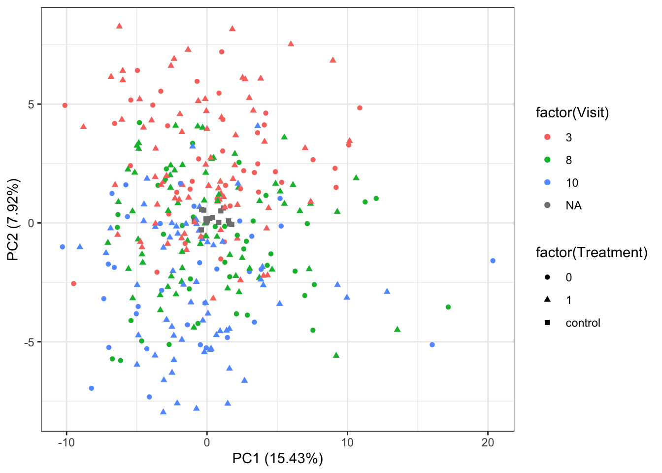
PC2 versus PC3
ggplot(plotTab, aes(x=PC2, y=PC3, shape = factor(Treatment), color= factor(Visit))) +
    geom_point() +
    xlab(sprintf("PC2 (%1.2f%%)",varExp[2])) +
    ylab(sprintf("PC3 (%1.2f%%)",varExp[3])) +
    theme_bw()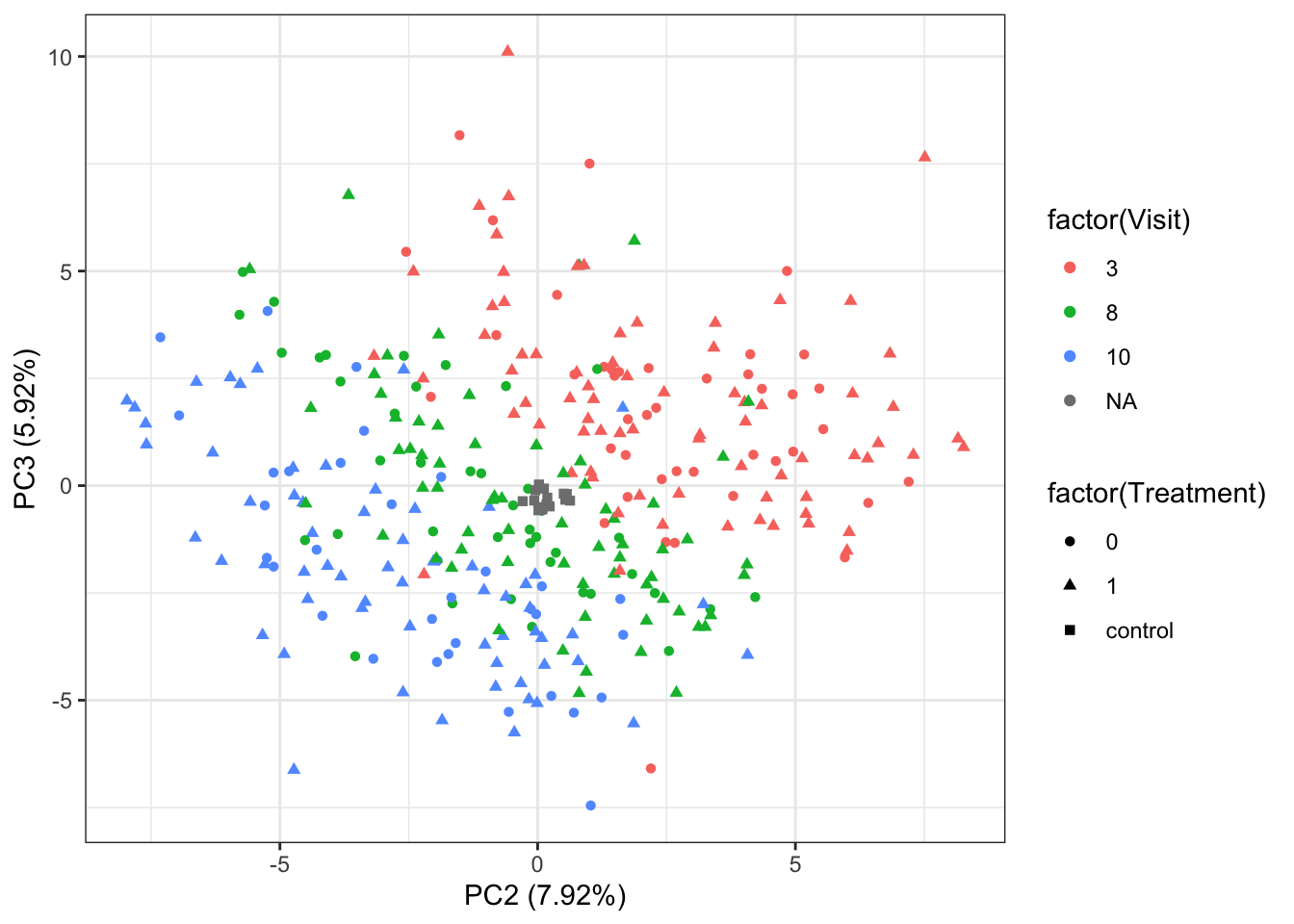
PC8 versus PC14 (separate treatment)
ggplot(plotTab, aes(x=PC8, y=PC14, shape = factor(Visit), color= factor(Treatment))) +
    geom_point() +
    xlab(sprintf("PC8 (%1.2f%%)",varExp[8])) +
    ylab(sprintf("PC14 (%1.2f%%)",varExp[14])) +
    theme_bw()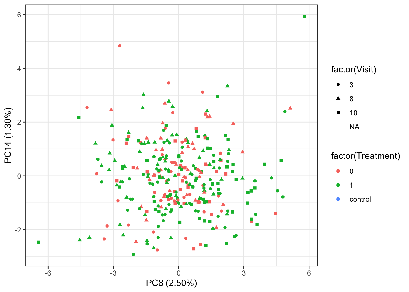
sessionInfo()R version 4.2.0 (2022-04-22)
Platform: x86_64-apple-darwin17.0 (64-bit)
Running under: macOS Big Sur/Monterey 10.16
Matrix products: default
BLAS: /Library/Frameworks/R.framework/Versions/4.2/Resources/lib/libRblas.0.dylib
LAPACK: /Library/Frameworks/R.framework/Versions/4.2/Resources/lib/libRlapack.dylib
locale:
[1] en_US.UTF-8/en_US.UTF-8/en_US.UTF-8/C/en_US.UTF-8/en_US.UTF-8
attached base packages:
[1] stats4 stats graphics grDevices utils datasets methods
[8] base
other attached packages:
[1] forcats_0.5.1 stringr_1.4.1
[3] dplyr_1.1.4.9000 purrr_0.3.4
[5] readr_2.1.2 tidyr_1.2.0
[7] tibble_3.2.1 ggplot2_3.4.1
[9] tidyverse_1.3.2 DEP_1.18.0
[11] SummarizedExperiment_1.26.1 Biobase_2.56.0
[13] GenomicRanges_1.48.0 GenomeInfoDb_1.32.2
[15] IRanges_2.30.0 S4Vectors_0.34.0
[17] BiocGenerics_0.42.0 MatrixGenerics_1.8.1
[19] matrixStats_0.62.0
loaded via a namespace (and not attached):
[1] utf8_1.2.4 shinydashboard_0.7.2 gmm_1.6-6
[4] tidyselect_1.2.1 RSQLite_2.2.15 AnnotationDbi_1.58.0
[7] htmlwidgets_1.5.4 grid_4.2.0 BiocParallel_1.30.3
[10] norm_1.0-10.0 maxstat_0.7-25 munsell_0.5.0
[13] codetools_0.2-18 preprocessCore_1.58.0 DT_0.23
[16] withr_3.0.0 colorspace_2.0-3 highr_0.9
[19] knitr_1.39 rstudioapi_0.13 ggsignif_0.6.3
[22] mzID_1.34.0 labeling_0.4.2 git2r_0.30.1
[25] slam_0.1-50 GenomeInfoDbData_1.2.8 KMsurv_0.1-5
[28] farver_2.1.1 bit64_4.0.5 rprojroot_2.0.3
[31] vctrs_0.6.5 generics_0.1.3 TH.data_1.1-1
[34] xfun_0.31 sets_1.0-21 R6_2.5.1
[37] doParallel_1.0.17 clue_0.3-61 locfit_1.5-9.6
[40] MsCoreUtils_1.8.0 bitops_1.0-7 cachem_1.0.6
[43] fgsea_1.22.0 DelayedArray_0.22.0 assertthat_0.2.1
[46] promises_1.2.0.1 scales_1.2.0 vroom_1.5.7
[49] multcomp_1.4-19 googlesheets4_1.0.0 gtable_0.3.0
[52] sva_3.44.0 Cairo_1.6-0 affy_1.74.0
[55] sandwich_3.0-2 workflowr_1.7.0 rlang_1.1.3
[58] genefilter_1.78.0 mzR_2.30.0 GlobalOptions_0.1.2
[61] splines_4.2.0 rstatix_0.7.0 gargle_1.2.0
[64] impute_1.70.0 hexbin_1.28.2 broom_1.0.0
[67] BiocManager_1.30.18 yaml_2.3.5 abind_1.4-5
[70] modelr_0.1.8 backports_1.4.1 httpuv_1.6.6
[73] tools_4.2.0 relations_0.6-12 affyio_1.66.0
[76] ellipsis_0.3.2 gplots_3.1.3 jquerylib_0.1.4
[79] RColorBrewer_1.1-3 MSnbase_2.22.0 Rcpp_1.0.9
[82] plyr_1.8.7 visNetwork_2.1.0 zlibbioc_1.42.0
[85] RCurl_1.98-1.7 ggpubr_0.4.0 GetoptLong_1.0.5
[88] cowplot_1.1.1 zoo_1.8-10 haven_2.5.0
[91] cluster_2.1.3 exactRankTests_0.8-35 fs_1.5.2
[94] magrittr_2.0.3 magick_2.7.3 data.table_1.14.8
[97] circlize_0.4.15 survminer_0.4.9 reprex_2.0.1
[100] googledrive_2.0.0 pcaMethods_1.88.0 mvtnorm_1.1-3
[103] ProtGenerics_1.28.0 shinyjs_2.1.0 hms_1.1.1
[106] mime_0.12 evaluate_0.15 xtable_1.8-4
[109] XML_3.99-0.10 readxl_1.4.0 gridExtra_2.3
[112] shape_1.4.6 compiler_4.2.0 KernSmooth_2.23-20
[115] ncdf4_1.19 crayon_1.5.2 htmltools_0.5.4
[118] mgcv_1.8-40 later_1.3.0 tzdb_0.3.0
[121] lubridate_1.8.0 DBI_1.1.3 dbplyr_2.2.1
[124] ComplexHeatmap_2.12.1 MASS_7.3-58 tmvtnorm_1.5
[127] jyluMisc_0.1.5 Matrix_1.5-4 car_3.1-0
[130] cli_3.6.2 vsn_3.64.0 imputeLCMD_2.1
[133] marray_1.74.0 parallel_4.2.0 igraph_1.3.4
[136] km.ci_0.5-6 pkgconfig_2.0.3 piano_2.12.0
[139] MALDIquant_1.21 xml2_1.3.3 foreach_1.5.2
[142] annotate_1.74.0 bslib_0.4.1 XVector_0.36.0
[145] drc_3.0-1 rvest_1.0.2 digest_0.6.30
[148] Biostrings_2.64.0 rmarkdown_2.14 cellranger_1.1.0
[151] fastmatch_1.1-3 survMisc_0.5.6 edgeR_3.38.1
[154] shiny_1.7.4 gtools_3.9.3 rjson_0.2.21
[157] nlme_3.1-158 lifecycle_1.0.4 jsonlite_1.8.3
[160] carData_3.0-5 limma_3.52.2 fansi_1.0.6
[163] pillar_1.9.0 lattice_0.20-45 KEGGREST_1.36.3
[166] fastmap_1.1.0 httr_1.4.3 plotrix_3.8-2
[169] survival_3.4-0 glue_1.7.0 png_0.1-7
[172] iterators_1.0.14 bit_4.0.4 stringi_1.7.8
[175] sass_0.4.2 blob_1.2.3 memoise_2.0.1
[178] caTools_1.18.2