Good scientific practice: Design of High Throughput Experiments and their Analysis
2023-01-17
Why are we here?
To consult the statistician after an experiment is finished is often merely to ask him to conduct a post mortem examination. He can perhaps say what the experiment died of.
Presidential Address to the First Indian Statistical Congress, 1938. Sankhya 4, 14-17.
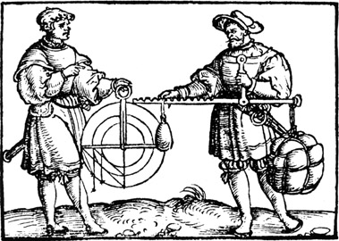
R.A. Fisher, Pioneer of Statistics and Experimental Design
Design of High Throughput Experiments
This lecture is based on Chapter 13 of the book
Modern Statistics for Modern Biology
by Susan Holmes, Wolfgang Huber
https://www.huber.embl.de/msmb/

Topics
- Resource allocation & experimental design: a matter of trade-offs & good judgement
- Dealing with the different types of variability; partitioning variability
- Experiments, studies, …
- Power, sample size and efficiency.
- Transformations
- Things to worry about: dependencies, batch effects, unwanted variation.
- Compression, redundancy and sufficiency
- Computational best practices

Accuracy vs precision
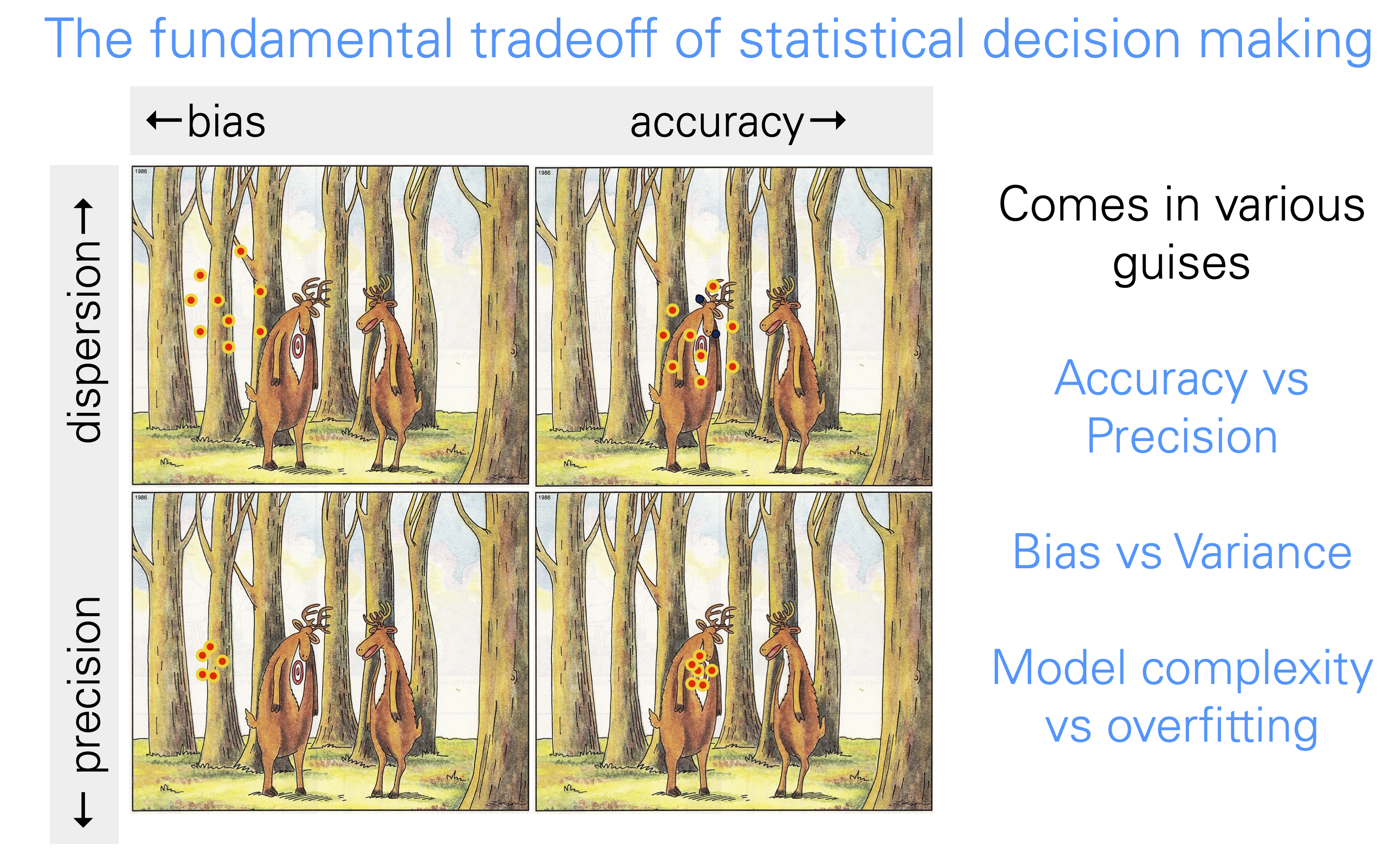
Illustration: experiment
Well-characterized cell line growing in laboratory conditions on defined media, temperature and atmosphere.
We administer a precise amount of a drug, and after 72h we measure the activity of a specific pathway reporter.

Illustration: challenges with studies
We recruit patients with a chronic disease and who fulfill inclusion criteria, and we ask them to take a drug each day exactly at 6 am. Before, and after 3 months, we perform a diagnostic test.
- People may forget to take the pill or take it at the wrong time.
- Some may feel that the disease got worse and stop taking the drug.

- Some may feel that the disease got better and stop taking the drug.
- Some may lead a healthy life-style, others drink, smoke and eat junk food.
- Maybe it’s not one disease but several
- And all of these factors may be correlated with each other in complex ways.
What to do about this?
- need much larger sample sizes than with an experiment
- randomization, blinding, documentation
Quiz
For reliable variant calling with current sequencing technology, you need ca. \(30\times\) coverage for a human genome.
In the 1000 Genomes Project, the average depth of the data produced was 5.1 for 1092 individuals. Why was that study design chosen?
\(\quad\)
\(\quad\)

Error models: Noise is in the eye of the beholder
The efficiency of most biochemical or physical processes involving nucleic acid polymers depends on their sequence content, for instance, occurrences of long homopolymer stretches, palindromes, GC content.
These effects are not universal, but can also depend on factors like concentration, temperature, which enzyme is used, etc.
When looking at RNA-Seq data, should we treat GC content as noise or as bias?
One person’s noise can be another’s bias

We may think that the outcome of tossing a coin is completely random.
If we meticulously registered the initial conditions of the coin flip and solved the mechanical equations, we could predict which side has a higher probability of coming up: noise becomes bias.
We use mathematical and probabilistic modelling as a method to bring some order into our ignorance—but keep in mind that such models are an expression of our subjective ignorance, not an objective property of the world.
A lack of units
Pre-modern measurement systems measured lengths in feet, ells, inches (first joint of an index finger), weights in stones, volumes in multiples of the size of a wine jar, etc.
In the International System of Units, meters, seconds, kilograms, amperes, … are defined based on universal physical constants.
There is no reliance on artefacts, and a meter measured by a lab in Canada using one instrument has the same meaning as a meter measured a year later by a lab in Heidelberg using a different instrument, by a space probe in the Kuiper belt, or by an extraterrestrial intelligence on Proxima Cen b.
Measurements in biology are, unfortunately, rarely that comparable.
Often, absolute values are not reported (these would require units), but only fold changes with regard to some local reference.
Even when absolute values exist (e.g., read counts in an RNA-Seq experiment) they usually do not translate into universal units such as molecules per cell or mole per milliliter.
What is a good normalization method?
- If the normalization is ‘off’, we can have increased variability between replicates
- … and/or apparent systematic differences between different conditions that are not real
- \(\to\) false positives, false negatives
What do we want from a good normalization method:
- remove technical variation
- but keep biological variation
Possible figure of merit?
- signal-to-noise ratio, computed from pos. and neg. controls, replicates
Occam’s razor

If one can explain a phenomenon without assuming this or that hypothetical entity, there is no ground for assuming it.
One should always opt for an explanation in terms of the fewest possible causes, factors, or variables.
Regular and catastrophic noise
Regular noise: can be modeled by simple probability models (independent normal, Poisson distributions; or mixtures such as Gamma-Poisson or Laplace)
Can use relatively straightforward methods to take regular noise into account
Real world is more complicated: measurements can be completely off the scale (sample swap, contamination, software bug, …)
Multiple errors often come together: e.g., a whole microtiter plate went bad, affecting all data measured from it.
Such events are hard to model or even correct for—our best chance is data quality assessment, outlier detection and documented removal.
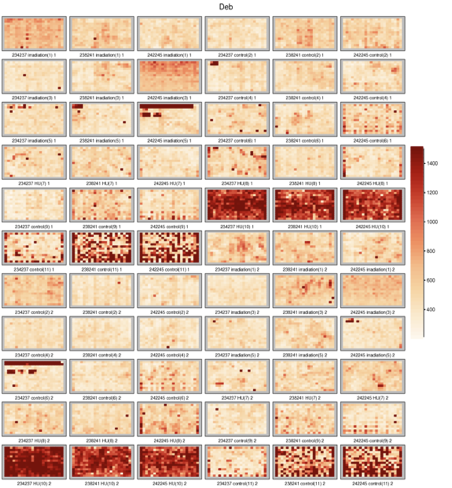
RNAi screen example
Keeping track: Dailies
![]()
A film director will view daily takes, to correct potential lighting, shooting issues before they affect too much footage. It is a good idea not to wait until all the runs of an experiment have been finished before looking at the data.
Intermediate data analyses and visualizations will track eventual unexpected sources of variation in the data and enable you to adjust the protocol.
It is important to be aware of sources of variation as they occur and adjust for them.
Vary one factor at a time


Ibn Sina’s Canon of Medicine (1020) lists seven rules of experimental design, including the need for controls and replication, the danger of confounding and the necessity of changing only one factor at a time.
This dogma was overthrown in the 20th century by RA Fisher.
A toy example: two-group comparison
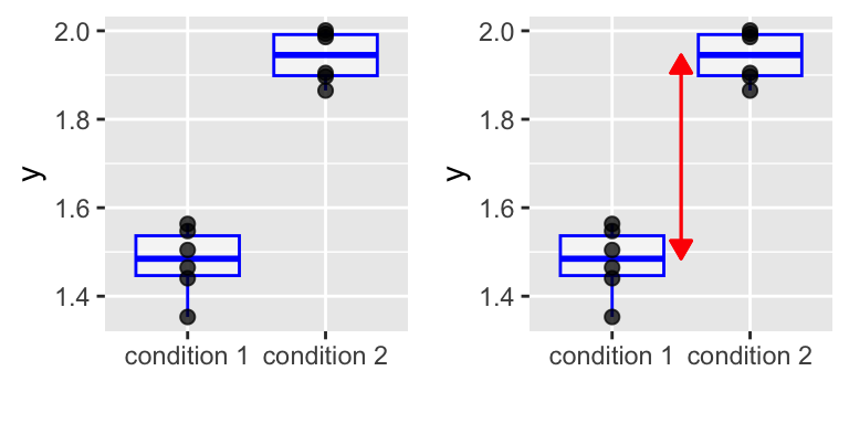
However, suppose the experiment was done in two “batches”, and we color the data according that:
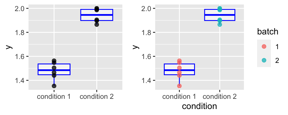
We cannot conclude because of confounding.
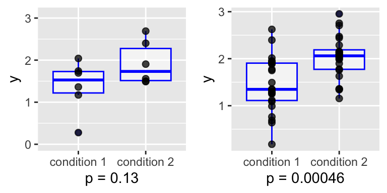
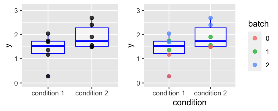
Now suppose there is no such fatal confounding, but an unknown batch effect that is balanced between the conditions, and effectively causes higher noise levels. Then, the previous sample size (2 x 6) is not enough. With 2 x 24, it looks better:
Decomposition of variability: analysis of variance (ANOVA)
lm(y ~ condition, data = df1) |> anova()Analysis of Variance Table
Response: y
Df Sum Sq Mean Sq F value Pr(>F)
condition 1 0.8828 0.8828 2.723 0.1299
Residuals 10 3.2420 0.3242 \(\quad\)
lm(y ~ condition + batch, data = df1) |> anova()Analysis of Variance Table
Response: y
Df Sum Sq Mean Sq F value Pr(>F)
condition 1 0.88280 0.88280 8.4591 0.019635 *
batch 2 2.40714 1.20357 11.5328 0.004398 **
Residuals 8 0.83489 0.10436
---
Signif. codes: 0 '***' 0.001 '**' 0.01 '*' 0.05 '.' 0.1 ' ' 1Blocking: the case of paired experiments.
Darwin’s Zea Mays experiment:
  pot pair  type height
1   I    a cross 23.500
2   I    a  self 17.375
3   I    b cross 12.000
4   I    b  self 20.375
5   I    c cross 21.000
6   I    c  self 20.000
pair
type a b c d e f g h i j k l m n o
cross 1 1 1 1 1 1 1 1 1 1 1 1 1 1 1
self 1 1 1 1 1 1 1 1 1 1 1 1 1 1 1- 15 pairs of plants, each with two different pollination methods, across 4 pots.
- a balanced design: all the different factor combinations have the same number of observation replicates.
- particularly easy to analyse
Paired t-test is equivalent to a 2-way ANOVA
with(darwin.maize,
  t.test(height[type == "self"], height[type == "cross"], paired = TRUE))
    Paired t-test

data:  height[type == "self"] and height[type == "cross"]
t = -2.148, df = 14, p-value = 0.0497
alternative hypothesis: true mean difference is not equal to 0
95 percent confidence interval:
 -5.229434169 -0.003899165
sample estimates:
mean difference
      -2.616667
fit = lm(height ~ type + pair, data = darwin.maize)
anova(fit)Analysis of Variance Table
Response: height
Df Sum Sq Mean Sq F value Pr(>F)
type 1 51.352 51.352 4.6139 0.0497 *
pair 14 86.264 6.162 0.5536 0.8597
Residuals 14 155.820 11.130
---
Signif. codes: 0 '***' 0.001 '**' 0.01 '*' 0.05 '.' 0.1 ' ' 1coef(fit)["typeself"] typeself
-2.616667 “Block what you can, randomize what you cannot”
(George Box, 1978)
Often we don’t know which nuisance factors will be important, or we cannot plan for them ahead of time.
In such cases, randomization is a practical strategy: at least in the limit of large enough sample size, the effect of any nuisance factor should average out.
Randomized Complete Block Design
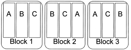
“The design space is divided into uniform units to account for any variation so that observed differences within units are largely due to true differences between treatments. Treatments are then assigned at random to the subjects in the blocks - once in each block. The defining feature of the Randomized Complete Block Design is that each block sees each treatment exactly once.” (Trudi Grant)
Randomization decreases bias
- Humans are bad at assigning treatments truly at random
- Random assignment reduces unconscious bias (special samples treated differently, “balancing things out”, …)
- Randomization also helps with unknown nuisance factors.
Randomization helps inference
- if the sample is randomly generated from a population, we can infer something about the population we drew from
Random does not mean haphazardly
- Need to use a random number generator and a seed.
There is also rich literature on deterministic, balanced block designs.
Effective sample size for dependent data.
A sample of independent observations is more informative than the same number of dependent observations. \(\Rightarrow\) Dependent data require larger samples. Intuition: each sample contains less information.
Consider an opinion poll. We knock at people’s doors and ask them a question.
- Scenario 1: pick \(n\) people at \(n\) random places throughout the country.
- Scenario 2: to save travel time, you pick \(n/3\) random places and then at each of these interview three people who live next door to each other.
In both cases, \(n\) people are polled is \(n\). But if we assume that people living in the same neighborhood are more likely to have similar opinions, the data from Scenario 2 are (positively) correlated.
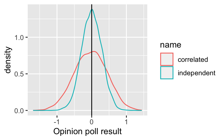
Simulation: “opinions” in a population of 100 people are \(N(0,1)\). We want to estimate the mean by sampling. In scenario 1, we ask 12 randomly selected people. In scenario, we ask 4 randomly selected people as well as two of their direct neighbours.
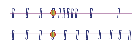
Time course: equalize the dependence structure by taking more frequent samples when there is more “going on”.
Data transformations
\[\begin{equation} X_{\text{obs}} = f(\theta) + \varepsilon \end{equation}\]
Homoskedastic: \(\quad\text{sd}(\varepsilon)=\text{const.}\)
Heteroskedastic: e.g.,
- multiplicative error: \(\quad\text{sd}(\varepsilon)\sim f(\theta)\)
- Poisson noise: \(\quad\text{var}(\varepsilon)\sim f(\theta)\)
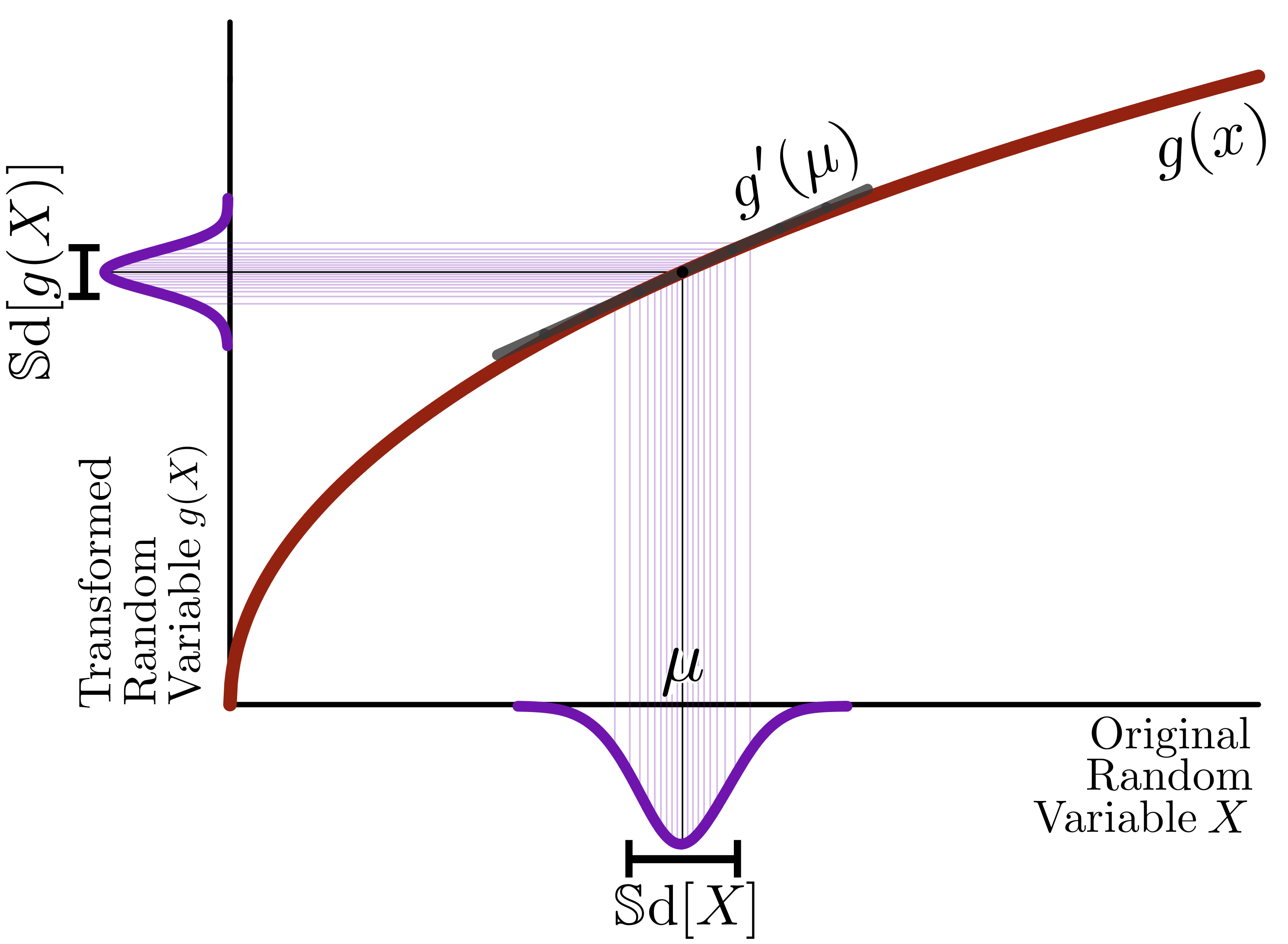
- multiplicative error: \(\log(X)\)
- Poisson noise: \(\sqrt X\)
Examples:
- Fluorescence based assays: additive + multiplicative (Rocke and Durbin 2001)
- RNA-Seq: Poisson + multiplicative.
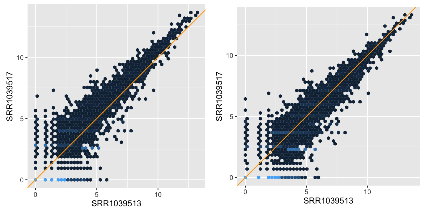
Data quality assessment and quality control
- QA: measure and monitor data quality
- QC: remove bad data
Pervade all phases of analysis: raw data, transformation, summarization, model fitting, hypothesis testing, screening for ‘’hits’’. Diagnostics and metrics:
- Feature value range (Boxplot, ECDF) across samples
- Joint distributions (scatter plots, heatmaps, sample-sample or feature-feature correlation matrices)?
- Correlation of replicates vs between biological conditions
- Evidence of batch effects (categorical, continuous)—–explicitly known or latent.
iSEE package: PBMC4k example, CYTOF example
MatrixQCVis package:
Henry Ford (possibly apocryphal): ‘’If I had asked people what they wanted, they would have said faster horses.’’: quality as fitness for purpose, versus adherence to specifications.
Not easy to nail down (or mathematically define) quality, the word is used with many meanings. See also http://en.wikipedia.org/wiki/Quality_(business)
Dichotomization is bad
Grouping / discretization of continuous variables

Dichotomizing continuous predictors in multiple regression: a bad idea
Royston, Altman, Sauerbrei
Statistics in Medicine 2006
Leaky pipelines and statistical sufficiency
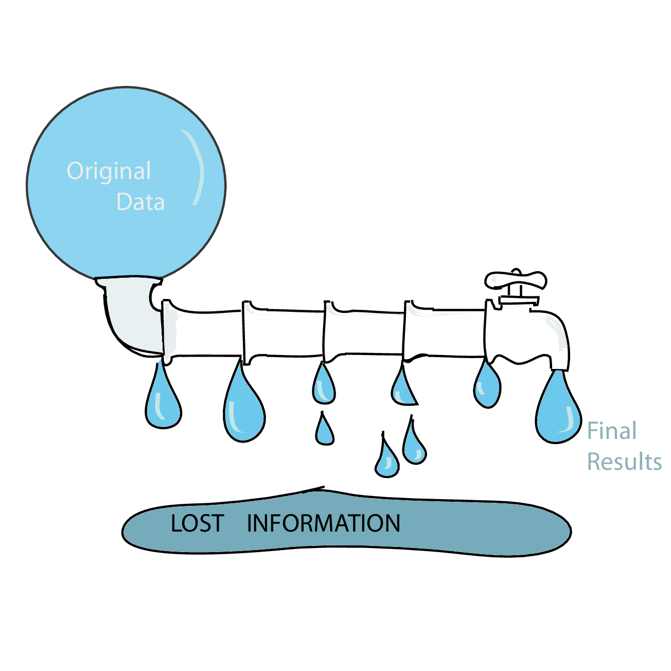
Data analysis pipelines in high-throughput biology often work as funnels that successively summarise and compress the data. In high-throughput sequencing, we may start with individual sequencing reads, then align them to a reference, then only count the aligned reads for each position, summarise positions to genes (or other kinds of regions), then “normalize” these numbers by library size, etc.
At each step, we loose some information, and it is important to make sure we still have enough information for the task at hand. The problem is particularly burning if we use a data pipeline built from a series of separate components without enough care being taken ensuring that all the information necessary for ulterior steps is conserved.
Statisticians have a concept for whether certain summaries enable the reconstruction of all the relevant information in the data: sufficiency. E.g., in a Bernoulli random experiment with a known number of trials, \(n\), the number of successes is a sufficient statistic for estimating the probability of success \(p\).
In a 4-state Markov chain (A,C,G,T) such as the one we saw in Lecture 2, what are the sufficient statistics for the estimation of the transition probabilities?
Iterative approaches akin to what we saw when we used the EM algorithm can sometimes help avoid information loss. For instance, when analyzing mass spectroscopy data, a first run guesses at peaks individually for every sample. After this preliminary spectra-spotting, another iteration allows us to borrow strength from the other samples to spot spectra that may have been labeled as noise.
Acknowledgments


Quarto sources for this talk: https://github.com/wolfganghuber/Best-Analysis-Practices-Talk
References
![]()