![]()
Analysis of variance, regression and testing
Wolfgang Huber

Analysis of variance
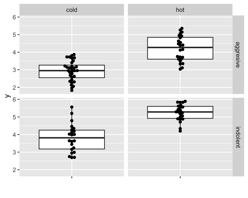
A set of observations
Standard deviation: 1.1.
Find an explanatory factor
Standard deviation: 0.8.
And another explanatory factor
Standard deviation: 0.7.
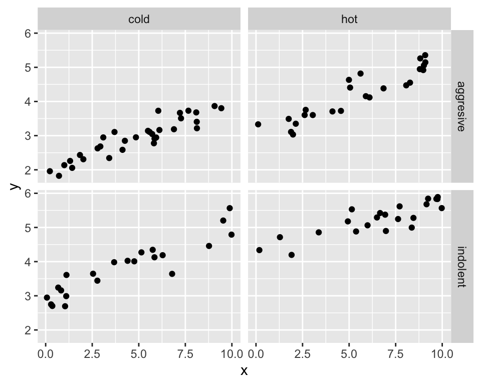
And another explanatory variable, this time continuous-valued
Residuals: \(y - \beta_1\,g1 - \beta_2\,g2 - \beta_3\,x\).
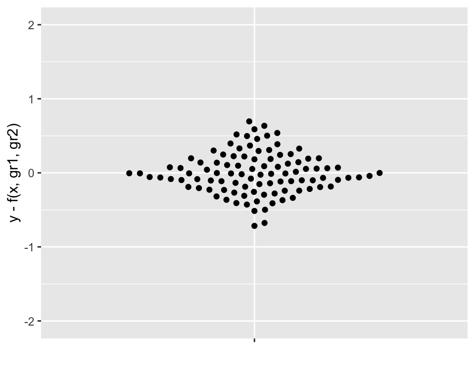
Standard deviation: 0.3.
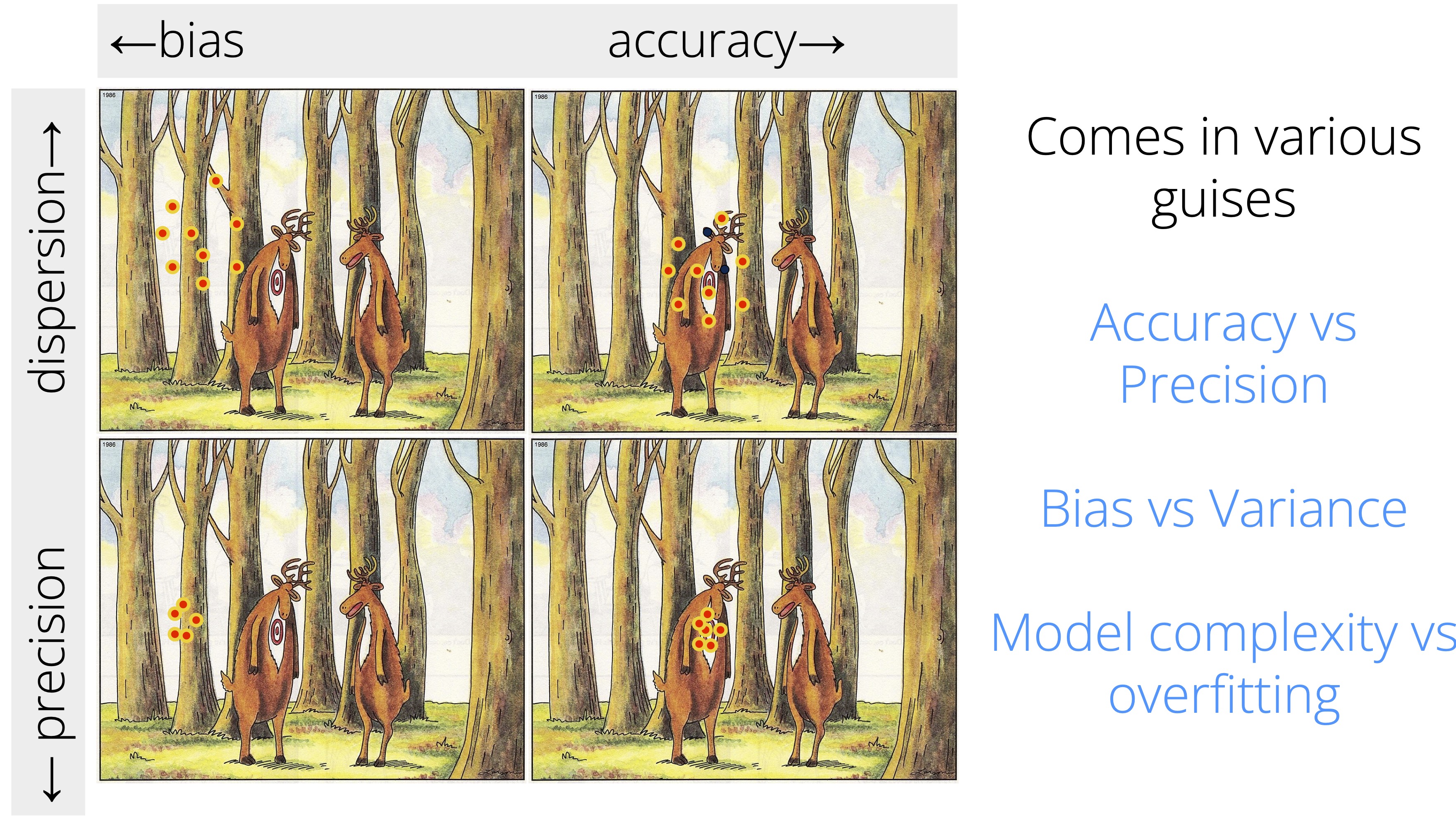
Basic idea of ANOVA
\[ \text{Overall variance} = \text{Signal component 1} + \text{Signal component 2} + \ldots + \text{Rest} \]
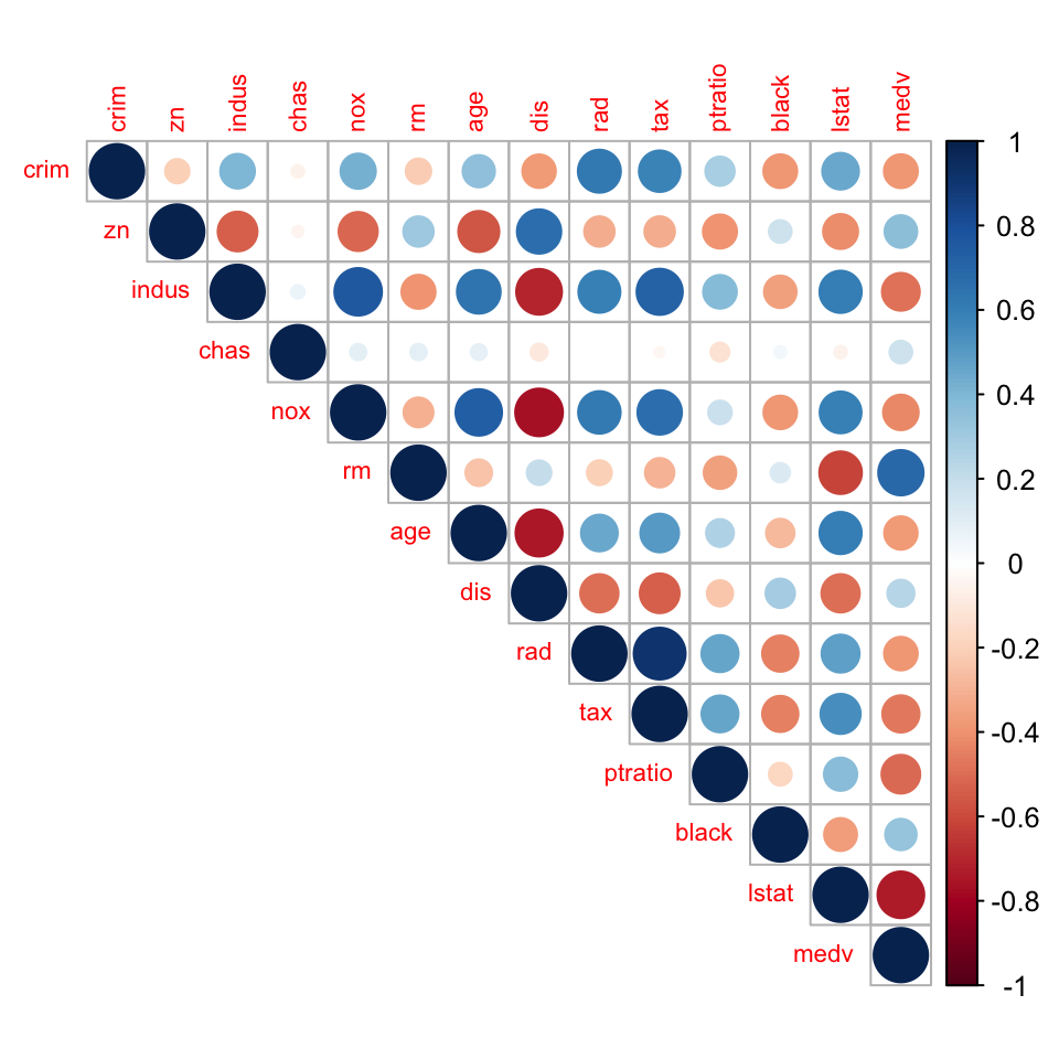
Colinearity, confounding
     crim zn indus chas   nox    rm  age    dis rad tax ptratio  black lstat medv
1 0.00632 18  2.31    0 0.538 6.575 65.2 4.0900   1 296    15.3 396.90  4.98 24.0
2 0.02731  0  7.07    0 0.469 6.421 78.9 4.9671   2 242    17.8 396.90  9.14 21.6
3 0.02729  0  7.07    0 0.469 7.185 61.1 4.9671   2 242    17.8 392.83  4.03 34.7
4 0.03237  0  2.18    0 0.458 6.998 45.8 6.0622   3 222    18.7 394.63  2.94 33.4
5 0.06905  0  2.18    0 0.458 7.147 54.2 6.0622   3 222    18.7 396.90  5.33 36.2
6 0.02985  0  2.18    0 0.458 6.430 58.7 6.0622   3 222    18.7 394.12  5.21 28.7
Housing Values in Suburbs of Boston. The Boston data frame has 506 rows and 14 columns.
| varname | meaning |
|---|---|
| nox | nitrogen oxides concentration (parts per 10 million) |
| rm | average number of rooms per dwelling |
| dis | weighted mean of distances to five Boston employment centres |
(Intercept)         dis          rm
-34.6360502 0.4888485 8.8014118 (Intercept) dis rm nox
-10.1181462 -0.6627196 8.0971906 -28.3432861 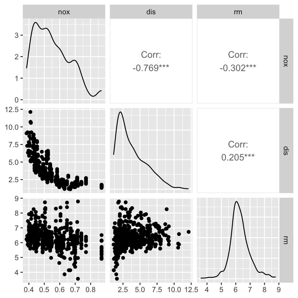
| varname | meaning |
|---|---|
| zn | proportion of residential land zoned for lots over 25,000 sq.ft |
| indus | proportion of non-retail business acres per town |
| chas | Charles River proximity (1 if tract bounds river; 0 otherwise) |
| nox | nitrogen oxides concentration (parts per 10 million) |
| rm | average number of rooms per dwelling |
| age | proportion of owner-occupied units built prior to 1940 |
| dis | weighted mean of distances to five Boston employment centres |
| rad | index of accessibility to radial highways |
| tax | full-value property-tax rate per $10,000 |
| ptratio | pupil-teacher ratio by town |
| black | \(1000(b−0.63)^2\), where \(b\) is the proportion of blacks |
| lstat | lower status of the population (percent) |
| medv | median value of owner-occupied homes in $1000s |
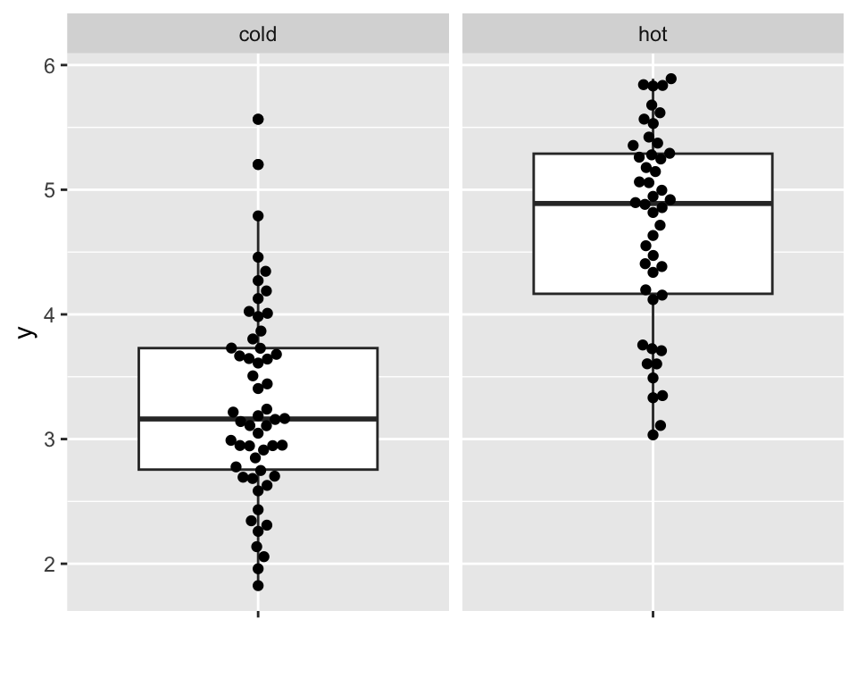
Blocking, pairing
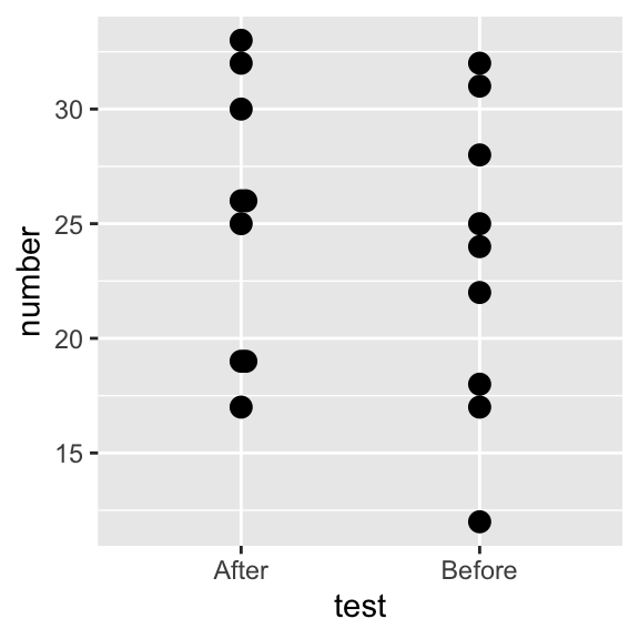
    Welch Two Sample t-test

data:  number by test
t = 0.67446, df = 15.736, p-value = 0.5098
alternative hypothesis: true difference in means between group After and group Before is not equal to 0
95 percent confidence interval:
 -4.29481  8.29481
sample estimates:
 mean in group After mean in group Before
            25.22222             23.22222
The p value is not “significant”.
Call:
lm(formula = number ~ test + subject, data = Fitness)

Residuals:
   Min     1Q Median     3Q    Max
-2.000 -0.875  0.000  0.875  2.000

Coefficients:
            Estimate Std. Error t value Pr(>|t|)
(Intercept)  31.0000     1.1487  26.988 3.83e-09 ***
testBefore   -2.0000     0.7265  -2.753  0.02494 *
subject2      2.0000     1.5411   1.298  0.23053
subject3    -12.0000     1.5411  -7.787 5.30e-05 ***
subject4     -6.0000     1.5411  -3.893  0.00459 **
subject5    -15.5000     1.5411 -10.058 8.13e-06 ***
subject6      1.0000     1.5411   0.649  0.53459
subject7     -5.0000     1.5411  -3.244  0.01180 *
subject8    -11.5000     1.5411  -7.462 7.18e-05 ***
subject9     -5.0000     1.5411  -3.244  0.01180 *
---
Signif. codes:  0 '***' 0.001 '**' 0.01 '*' 0.05 '.' 0.1 ' ' 1

Residual standard error: 1.541 on 8 degrees of freedom
Multiple R-squared:  0.9708,    Adjusted R-squared:  0.938
F-statistic: 29.57 on 9 and 8 DF,  p-value: 3.356e-05
The p value for testBefore (=difference before - after) is “significant”.
    Paired t-test

data:  FitnessW$After and FitnessW$Before
t = 2.753, df = 8, p-value = 0.02494
alternative hypothesis: true mean difference is not equal to 0
95 percent confidence interval:
 0.3247268 3.6752732
sample estimates:
mean difference
2 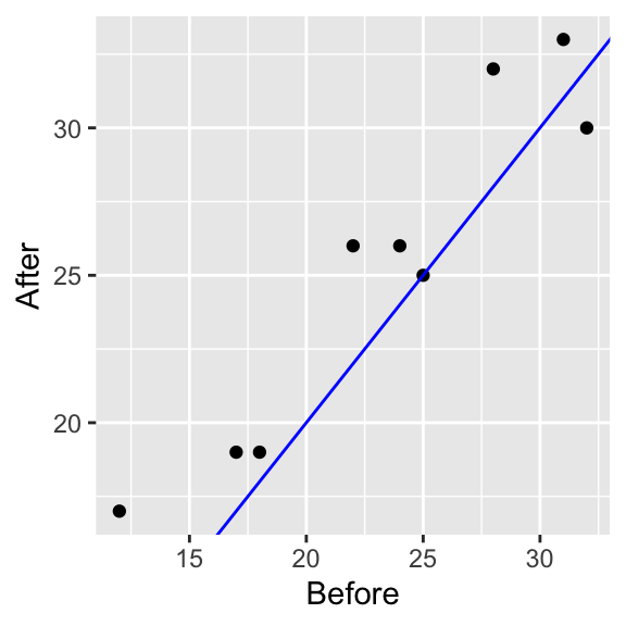
The paired \(t\)-test is the same as the linear model with subject as a covariate.
Generalizations
\[ y = \beta \cdot x + \varepsilon \]
Logistic regression
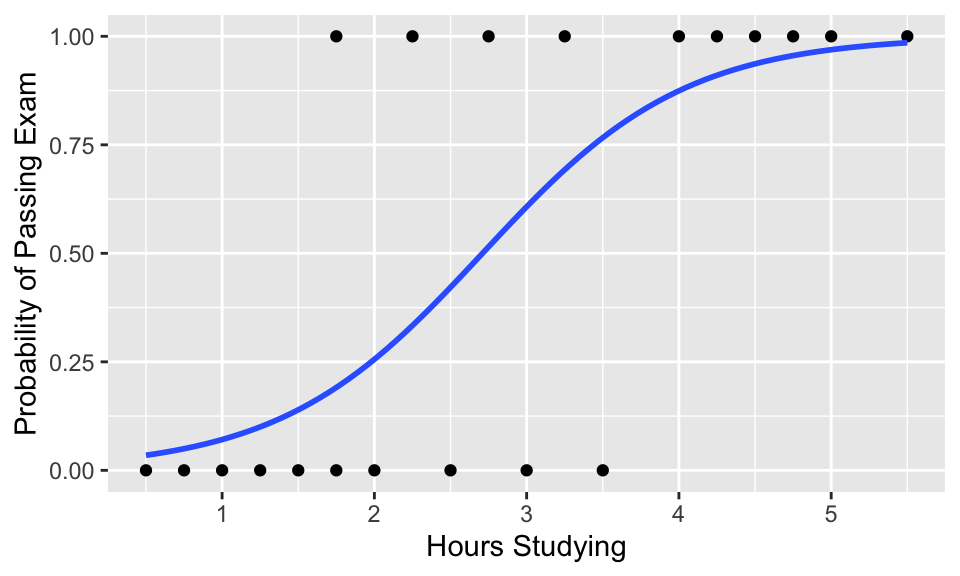
\[ \log\frac{p}{1-p} = \beta \cdot x \]
Generalized Linear Models
- Model \(\beta \cdot x\),
- (optional:) transform with a “link function” (e.g., \(\exp\)),
- insert the result as parameter into a statistical distribution.
Splines
(…)
Gaussian processes
In a Bayesian view of linear regression, we assume the data is generated from a linear function with some Gaussian noise:
\[ y = \mathbf{x}^\top \mathbf{w} + \epsilon, \quad \epsilon \sim \mathcal{N}(0, \sigma^2) \] We place a prior on the weights,
\[ \mathbf{w} \sim \mathcal{N}(0, \tau^2 I), \]
and this leads to a Gaussian prior over functions \(f(\mathbf{x}) = \mathbf{x}^\top \mathbf{w}\). When we marginalize over \(\mathbf{w}\), the function values at input points follow a multivariate Gaussian distribution.
A Gaussian Process can be seen as an infinite-dimensional generalization of the above.
- Instead of explicitly parameterizing functions with a finite weight vector \(\mathbf{w}\), we define a distribution over functions directly.
- A GP is fully specified by its mean function \(m(\mathbf{x})\) and covariance function (kernel) \(k(\mathbf{x}, \mathbf{x}')\).
Formally:
\[ f(\mathbf{x}) \sim \mathcal{GP}(m(\mathbf{x}), k(\mathbf{x}, \mathbf{x}')) \]
In fact, if you choose a linear kernel:
\[ k(\mathbf{x}, \mathbf{x}') = \mathbf{x}^\top \mathbf{x}' \]
then the GP reduces to Bayesian linear regression.
GPs are more powerful
- By choosing nonlinear kernels (e.g. RBF, Matérn), GPs can represent nonlinear functions while still retaining the analytical tractability of Gaussian distributions.
- This makes them nonparametric models—unlike linear regression which has a fixed number of parameters, GPs can adapt complexity to the data.
Hypothesis testing — why?
Test efficacy of a drug on people
- not an experiment — no complete control
- finite sample size
Prioritise results from a biological high-throughput experiment
- e.g., RNA-seq differential expression
- CRISPR screen
Understand impact of humidity on prevalence of leptospirosis
- No understanding of mechanism involved / needed / desired
- Wouldn’t we want to use any available understanding or ‘priors’?

Fundamental tradeoffs in statistical decision making
Basic problem: making binary decision
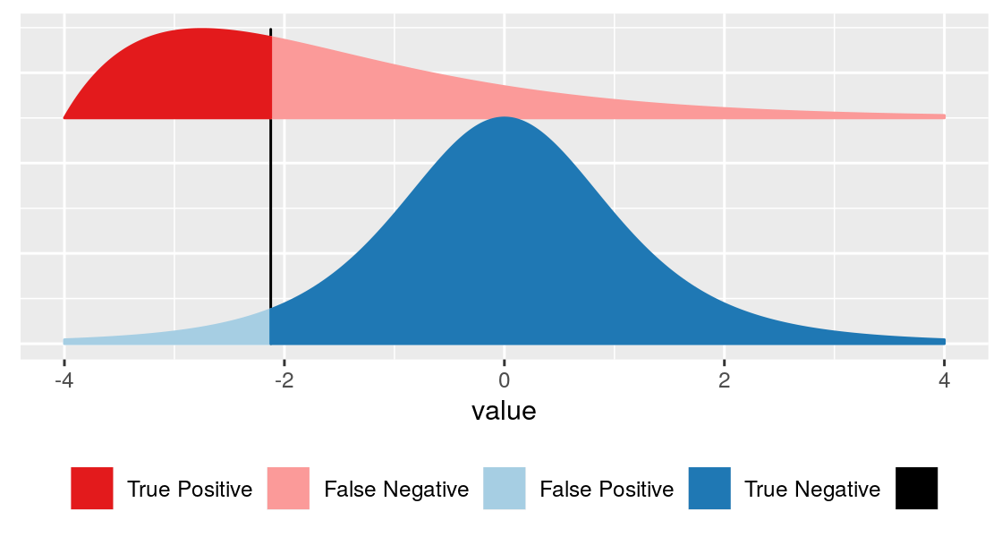
False discovery rate \[ \text{FDR} = \frac{\text{area shaded in light blue}}{\text{sum of areas to left of vertical bar (light blue + dark red)}} \]
For this, we need to know:
- blue curve: how is \(x\) distributed if no effect
- red curve: how is \(x\) distributed if there is effect
- the relative sizes of the blue and the red classes
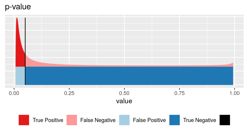
Basic problem: making binary decision
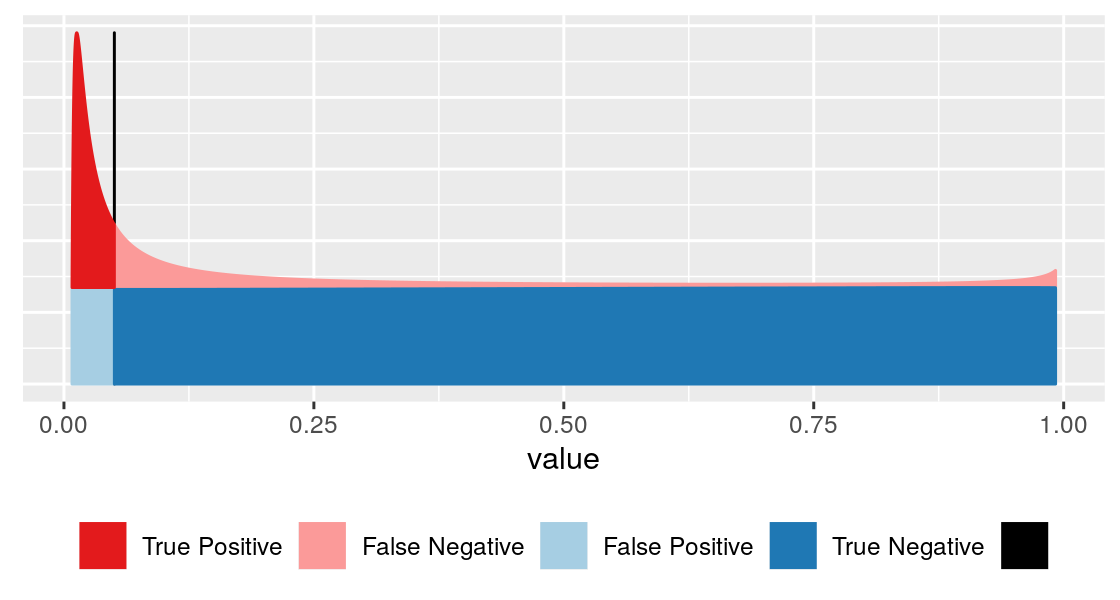
\[ \text{p} = \frac{\text{area shaded in light blue}}{\text{sum of the blue areas (=1)}} \]
For this, we need to know:
- how is \(x\) distributed if no effect

| Hypothesis testing | Machine Learning |
|---|---|
| Some theory/model and no or few parameters | Lots of free parameters |
| No training data | Lots of training data |
| More rigid/formulaic | Using multiple variables |
| Regulatory use | … or objects that are not even traditional variables (kernel methods, DNN) |
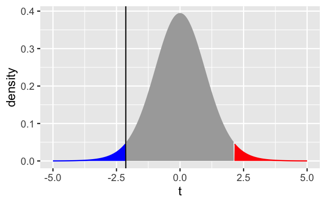
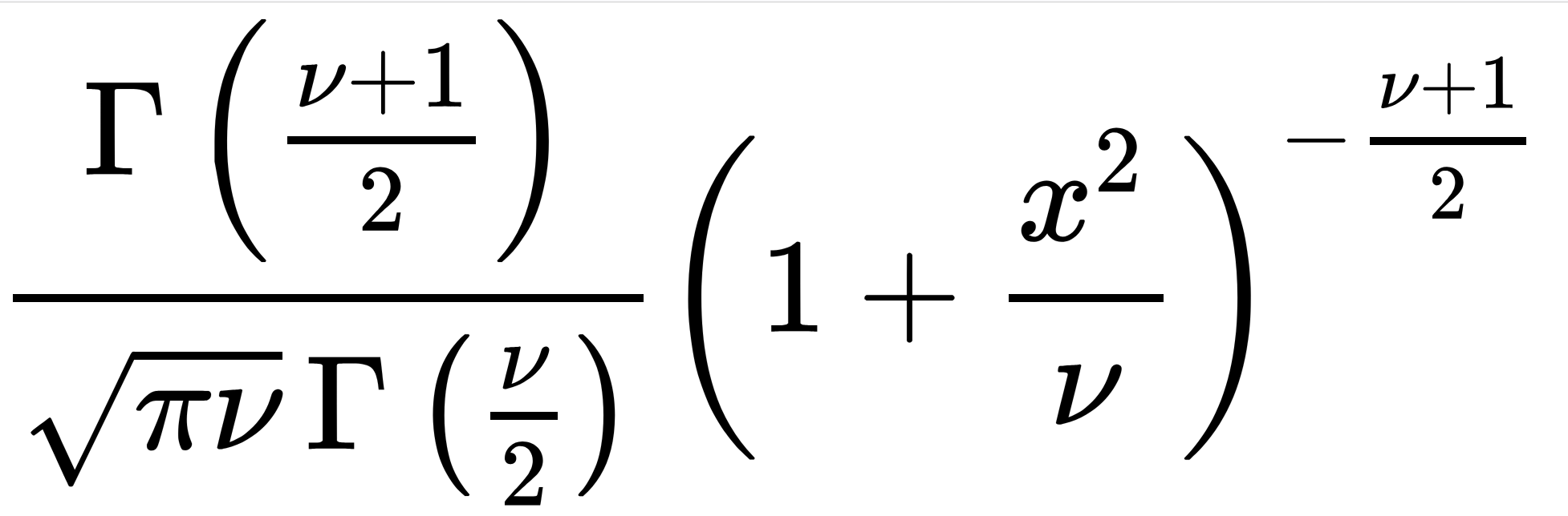
Comparing two groups: the \(t\)-statistic
For univariate real-valued data


Parametric Theory vs Simulation