Analysis of the new DIA proteomics data
Junyan Lu
Last updated: 2024-11-26
Checks: 4 2
Knit directory: RA_Tcell_omics/analysis/
This reproducible R Markdown analysis was created with workflowr (version 1.7.0). The Checks tab describes the reproducibility checks that were applied when the results were created. The Past versions tab lists the development history.
Great job! The global environment was empty. Objects defined in the global environment can affect the analysis in your R Markdown file in unknown ways. For reproduciblity it’s best to always run the code in an empty environment.
The command set.seed(20221110) was run prior to running
the code in the R Markdown file. Setting a seed ensures that any results
that rely on randomness, e.g. subsampling or permutations, are
reproducible.
Great job! Recording the operating system, R version, and package versions is critical for reproducibility.
- unnamed-chunk-3
To ensure reproducibility of the results, delete the cache directory
DIA_proteomics_analysis_cache and re-run the analysis. To
have workflowr automatically delete the cache directory prior to
building the file, set delete_cache = TRUE when running
wflow_build() or wflow_publish().
Great job! Using relative paths to the files within your workflowr project makes it easier to run your code on other machines.
Tracking code development and connecting the code version to the
results is critical for reproducibility. To start using Git, open the
Terminal and type git init in your project directory.
This project is not being versioned with Git. To obtain the full
reproducibility benefits of using workflowr, please see
?wflow_start.
Load libraries and dataset
Analysis of the new DIA proteomic dataset
seProt <- maeObj[["Proteome_DIA"]]
dim(seProt)
[1] 5450 15Heatmap visualization
library(pheatmap)
#select top 1000 most variant
colAnno <- colData(seProt)[,c(1:13,19)] %>% data.frame()

protMat <- assays(seProt)[["imputed"]]
sds <- genefilter::rowSds(protMat)
#protMat <- protMat[order(sds, decreasing = T)[1:5000],]

pheatmap(protMat, show_rownames = FALSE, scale = "row",
         annotation_col = colAnno,
         clustering_method = "ward.D2")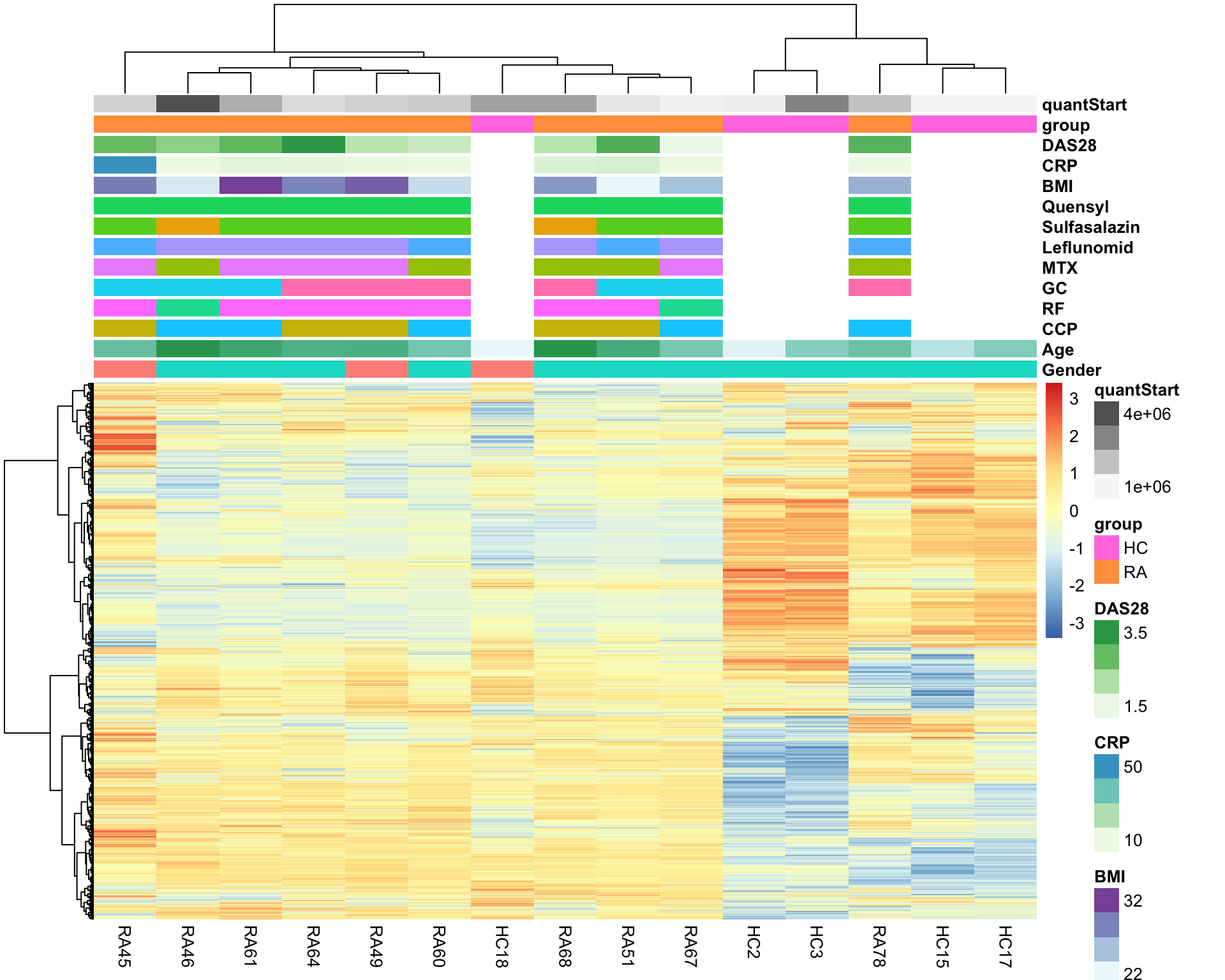
PCA
prRes <- prcomp(t(protMat), scale. = TRUE, center = TRUE)
plotTab <- prRes$x %>% as_tibble(rownames = "sampleID") %>%
left_join(as_tibble(colAnno, rownames = "sampleID"))
ggplot(plotTab, aes(x=PC1, y=PC2, col = group)) +
geom_point(size=5) +
ggrepel::geom_text_repel(aes(label = sampleID))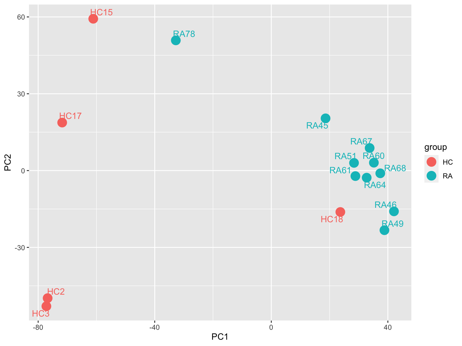 One HC sample HC18 is very close to RA samples. One RA
sample, RA78, is close to HC samples. Possible sample
swaping or purity issues?
One HC sample HC18 is very close to RA samples. One RA
sample, RA78, is close to HC samples. Possible sample
swaping or purity issues?
Correlate PCs with metadata
pcTest <- prRes$x[,1:10] %>%
    as_tibble(rownames = "sampleID")


metaTab <- colData(seProt)[,c(1:13,19)] %>%
   as_tibble(rownames = "sampleID")

resTab <- jyluMisc::testAssociation(pcTest, metaTab, joinID = "sampleID", plot = TRUE,
                                    onlySignificant = FALSE)

resTab$plot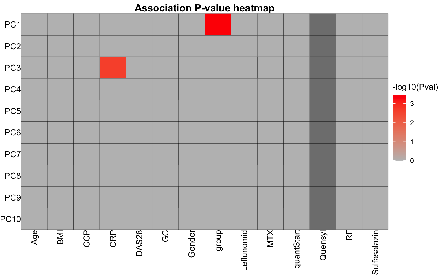
Differential expression using proDA
Differential protein expression using proDA, blocked for buffer condition
library(proDA)
protMat <- assays(seProt)[["norm"]]
designMat <- model.matrix(~ group , colData(seProt))
fit <- proDA(protMat, design = designMat)

resTab <- test_diff(fit, contrast = "groupRA") %>%
  arrange(pval) %>%
  mutate(symbol = rowData(seProt[name,])$symbol)

resTab_prot <- resTab
Warning: The above code chunk cached its results, but
it won’t be re-run if previous chunks it depends on are updated. If you
need to use caching, it is highly recommended to also set
knitr::opts_chunk$set(autodep = TRUE) at the top of the
file (in a chunk that is not cached). Alternatively, you can customize
the option dependson for each individual chunk that is
cached. Using either autodep or dependson will
remove this warning. See the
knitr cache options for more details.
hist(resTab$pval)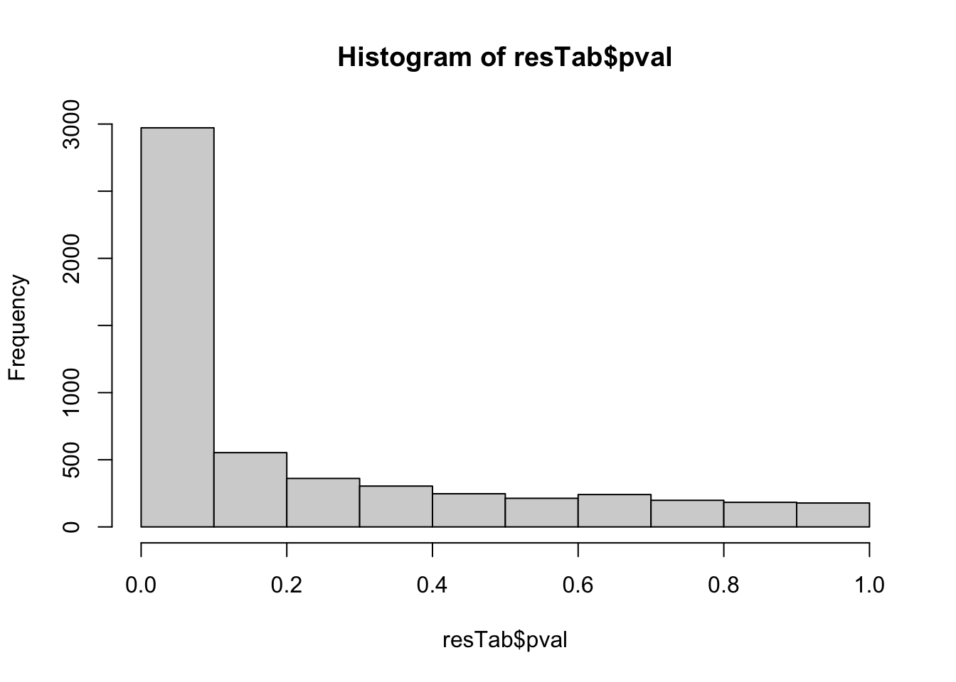 Quite strong difference can be detected.
Proteins with 5% FDR
resTab.sig <- filter(resTab, adj_pval < 0.05)
resTab.sig %>% select(symbol, pval, adj_pval, diff) %>%
  mutate_if(is.numeric, formatC, digits=1) %>%
  DT::datatable()
Plot top 9 examples
pList <- lapply(seq(9), function(i) {
  rec <- resTab.sig[i,]
  plotTab <- tibble(expr = protMat[rec$name,],
                    group = seProt$group)
  ggplot(plotTab, aes(x=group, y=expr)) +
    geom_boxplot(outlier.shape = NA) +
    ggbeeswarm::geom_quasirandom(aes(color = group), size=3) +
    ggtitle(rec$symbol) +
    theme_bw()
})

cowplot::plot_grid(plotlist = pList,ncol=3)
Enrichment analysis
gmts = list(Immune= "~/EMBL_projects/data/commonFiles/c7.immunesigdb.v2023.1.Hs.symbols.gmt",
            KEGG = "~/EMBL_projects/data/commonFiles/c2.cp.kegg.v6.2.symbols.gmt",
            C6 = "~/EMBL_projects/data/commonFiles/c6.all.v6.2.symbols.gmt",
            GOBP = "~/EMBL_projects/data/commonFiles/c5.bp.v6.2.symbols.gmt")

enRes <- runGeneSetEnrichment(resTab = resTab, gmts = gmts, method = "gsea",
                              collapsePathway = TRUE, genePCut = 1, pCutSet = 0.05)

ggsave(plot = enRes$plot, file = "../docs/enrichment_plots_DIA.pdf", height = 60, width = 30, limitsize = FALSE)Only use immune genesets related to CD8 T-cells
gmts = list(Immune= "~/EMBL_projects/data/commonFiles/c7.immunesigdb.v2023.1.Hs.symbols.gmt")

enRes <- runGeneSetEnrichment(resTab = resTab, gmts = gmts, method = "gsea", pathwayFilterKey = "CD8_TCELL",
                              collapsePathway = FALSE, genePCut = 1, pCutSet = 0.1, setFdr = TRUE)

ggsave(plot = enRes$plot, file = "../docs/enrichment_plots_TCELL_DIA.pdf", height = 10, width = 25, limitsize = FALSE)Write CSV output
write_csv2(select(resTab, symbol, diff, pval, adj_pval) %>% dplyr::rename(logFC = diff), "../docs/protein_P_values_DIA.csv")
write_csv2(as_tibble(protMat, rownames = "id") %>%
             mutate(symbol = rowData(seProt)[id,]$symbol) %>%
select(-id), "../docs/protein_normalized_abundance_DIA.csv")Association between protein expression and enhancer methylation levels
Are there any overlap between differential expressed proteins and differential methylated enhancer CpGs for the same protein?
#get significant protiens
resTab_prot <- resTab_prot %>%
  filter(pval < 0.01) %>%
  dplyr::rename(fc.prot = diff, p.prot = pval, padj.prot = adj_pval, protID = name) %>%
  select(protID, symbol, fc.prot, p.prot, padj.prot)

#get significant enhancer CpGs list
load("../output/resTab_enhancerCpG.RData")
resTab_enhancerCpG <- filter(resTab_enhancerCpG, P.Value < 0.01) %>%
  select(-B, -symbol) %>% dplyr::rename(p.cpg = P.Value, padj.cpg = adj.P.Val, fc.cpg = logFC, fc.cpg.beta = logFC_beta, symbol = gene)

#Get DMR regions
dmrRes <- readxl::read_xlsx("../docs/DMR_GeneHancer.xlsx") %>% filter(p.value < 0.01) %>%
  dplyr::rename(fc.dmr = estimate, p.dmr = p.value, padj.dmr = p.adjust, symbol = gene) %>%
  select(-c(enhancerId, feature, chr, start, end)) %>%
  arrange(p.dmr) %>% distinct(symbol,.keep_all = TRUE)

resTab.com <- resTab_enhancerCpG %>% left_join(resTab_prot, by ="symbol") %>%
  left_join(dmrRes, by = "symbol") %>%
  filter(!is.na(p.prot), !is.na(p.cpg))
Overlapped proteins
unique(sort(resTab.com$symbol)) [1] "ACAT2" "AKT1" "AKT2" "ALDOA" "AP2S1" "APOE" "ARID1A"
[8] "CAB39" "CASP9" "CBL" "CBR4" "CCL5" "CD84" "CDK9"
[15] "CHMP6" "COL6A1" "COPS6" "CTCF" "CTPS1" "D2HGDH" "DNMT1"
[22] "ECHS1" "FAHD1" "FAS" "FASN" "GAPVD1" "GOT1" "GPS1"
[29] "GPX1" "GPX4" "GZMB" "H6PD" "HACD2" "HPRT1" "HSD17B8"
[36] "HSPE1" "KRAS" "MAP2K3" "MAPK1" "NDUFA11" "NDUFA2" "NFS1"
[43] "NPM1" "NUP62" "OGDH" "PDGFB" "PDK1" "PFKL" "PGD"
[50] "PIK3CB" "PNP" "PPM1A" "PRKAA1" "PRKAB1" "PRKAG2" "PSMD13"
[57] "PTEN" "PTPRC" "RBBP5" "RUNX1" "SDHB" "SLC16A3" "STAT3"
[64] "STK3" "TFAM" "TFRC" "TYMP" "VPS28" "YWHAZ" Full table
resTab.com %>% mutate_if(is.numeric, formatC, digits=2) %>% DT::datatable()How many enhancer CpGs are associated with protein expression for each protein
plotTab <- resTab.com %>%
  mutate(direction = ifelse(fc.cpg*fc.prot >0, "same","opposite")) %>%
  group_by(symbol, direction) %>%
  summarise(n=length(probe)) %>% ungroup() %>%
  arrange(desc(n)) %>% mutate(symbol = factor(symbol, levels = unique(symbol)))

ggplot(plotTab, aes(x=symbol, y=n, fill = direction)) +
  geom_bar(stat = "identity") +
  theme(axis.text.x = element_text(angle = 90, hjust = 1, vjust = 0.5)) +
   ylab("Number of enhancer CpGs associated with RA phenotype") +
  xlab("")
direction means the whether the methylation level
change and protein expression change in RA versus healthy has the same
direction (both down- or up-regulated in RA samples) or the opposite
(one down-regulated and one up-regulated or vice versa).
direction means the whether the methylation level
change and protein expression change in RA versus healthy has the same
direction (both down- or up-regulated in RA samples) or the opposite
(one down-regulated and one up-regulated or vice versa).
Pathway enrichment analysis for those ~70 proteins (Fisher test)
Use all detected proteins as the background
gmts = list(Immune= "~/EMBL_projects/data/commonFiles/c7.immunesigdb.v2023.1.Hs.symbols.gmt",
            KEGG = "~/EMBL_projects/data/commonFiles/c2.cp.kegg.v6.2.symbols.gmt",
            C6 = "~/EMBL_projects/data/commonFiles/c6.all.v6.2.symbols.gmt",
            GOBP = "~/EMBL_projects/data/commonFiles/c5.bp.v6.2.symbols.gmt")

refList <- unique(rowData(seProt)$symbol)
geneList <- unique(sort(resTab.com$symbol))
fisherRes <- lapply(names(gmts), function(setName) {
  gmtFile <- gmts[[setName]]
  if (setName == "Immune") {
    pathKey <- "CD8_TCELL"
  } else pathKey = NULL
  res <- runFisher(geneList, refList, gmtFile, pathwayFilterKey = pathKey) %>%
    mutate(setName = setName)
}) %>%
  bind_rows()
Show significant results as a table (10% FDR)
fisherRes.sig <- filter(fisherRes, padj < 0.1)
fisherRes.sig %>% select(setName, TermID, pval, padj, genes, all) %>%
  dplyr::rename(Pathway = TermID, geneNum = genes, setSize = all) %>%
  mutate_if(is.numeric, formatC, digits=2) %>%
  DT::datatable()
Note that the enhancer CpGs were already filtered for manually specified interested genes, this enrichment results could just be because the list of interested genes provided by Franziska was already enriched for those pathways. Therefore, in the below analysis, I will also use this list as the background to avoid bias
Use the manually selected proteins provided by Franziska as the background.
gmts = list(Immune= "~/EMBL_projects/data/commonFiles/c7.immunesigdb.v2023.1.Hs.symbols.gmt",
            KEGG = "~/EMBL_projects/data/commonFiles/c2.cp.kegg.v6.2.symbols.gmt",
            C6 = "~/EMBL_projects/data/commonFiles/c6.all.v6.2.symbols.gmt",
            GOBP = "~/EMBL_projects/data/commonFiles/c5.bp.v6.2.symbols.gmt")

geneList <- unique(sort(resTab.com$symbol))
refList <- unique(readxl::read_excel("../data/Targeted-Methylation.xlsx", col_names = TRUE)[[1]])
fisherRes <- lapply(names(gmts), function(setName) {
  gmtFile <- gmts[[setName]]
  if (setName == "Immune") {
    pathKey <- "CD8_TCELL"
  } else pathKey = NULL
  res <- runFisher(geneList, refList, gmtFile, pathwayFilterKey = pathKey) %>%
    mutate(setName = setName)
}) %>%
  bind_rows()
Show significant results as a table (25% FDR)
fisherRes.sig <- filter(fisherRes, padj < 0.25)
fisherRes.sig %>% select(setName, TermID, pval, padj, genes, all) %>%
  dplyr::rename(Pathway = TermID, geneNum = genes, setSize = all) %>%
  mutate_if(is.numeric, formatC, digits=2) %>%
  DT::datatable()
No pathways passed 10% FDR.
Are there direct correlations between protein expression and their enhancer CpG methylation?
Prepare data
Methylation
load("../output/methData_20221118.RData")
methSub <- methData[resTab.com$probe,]
methMat <- assays(methSub)[["M"]]
colnames(methMat) <- methSub$Sample_Name
Protein expression
protMat <- assays(seProt)[["norm"]]Overlap
overSample <- intersect(colnames(methMat), colnames(protMat))
methMat <- methMat[,overSample]
protMat <- protMat[,overSample]
Correlation test
corResTab <- lapply(seq(nrow(resTab.com)), function(i) {
  rec <- resTab.com[i, ]
  methVal <- methMat[rec$probe,]
  protVal <- protMat[rec$protID,]
  res <- cor.test(methVal, protVal, use = "pairwise.complete.obs")
  tibble(protID = rec$protID, symbol = rec$symbol, probe = rec$probe, p.corr = res$p.value, coef.corr = res$estimate)
}) %>% bind_rows() %>% arrange(p.corr) %>%
  mutate(padj.corr = p.adjust(p.corr, method = "BH"))
Plot all significant correlations (P-value <0.05)
corResTab.sig <- filter(corResTab, p.corr <= 0.05) %>% arrange(symbol)
pList <- lapply(seq(nrow(corResTab.sig)), function(i) {
  rec <- corResTab.sig[i, ]
  plotTab <- tibble(sampleID = colnames(methMat),
                    methVal = methMat[rec$probe,],
                    protVal = protMat[rec$protID,]) %>%
    mutate(group = seProt[,sampleID]$group)

  ggplot(plotTab, aes(x=methVal, y=protVal)) +
    geom_point(aes(col = group)) +
    geom_smooth(method = "lm", se=FALSE) +
    ggtitle(sprintf("%s ~ %s (P=%s)", rec$symbol, rec$probe, formatC(rec$p.corr, digits = 1))) +
    ylab("Protein expression") + xlab("Methylation level (M-value)")

})
cowplot::plot_grid(plotlist = pList, ncol=3)
Are there any correlations between protein expressions and metabolites associated with RA?
Process metabolic data
seMeta <- maeObj[["Metabolism"]]
#glog transformation
metaMat <- glog(assay(seMeta))
Select metabolites passed P < 0.05
sigList <- read_csv2("./metabolite_P_values.csv")
metaMat <- metaMat[rownames(metaMat) %in% filter(sigList, P.Value < 0.05)$metabolite,]
rownames(metaMat)
[1] "2-OH-GA" "alpha Ketoglutarate" "Malate"
[4] "Succinate" metaTab <- as_tibble(metaMat, rownames = "metabolite") %>%
pivot_longer(-metabolite, names_to = "sampleID", values_to = "metaVal")Correlate protein expressions with these three metabolites
protMat <- assays(seProt[resTab.com$protID,])[["norm"]]

testTab <- as_tibble(protMat, rownames = "protID") %>%
  pivot_longer(-protID, names_to = "sampleID", values_to  = "protVal") %>%
  full_join(metaTab, by = "sampleID") %>%
  filter(!is.na(protVal),!is.na(metaVal)) %>%
  distinct(protID, sampleID, metabolite, .keep_all = TRUE)

resTab <- group_by(testTab, protID, metabolite) %>%
  nest() %>%
  mutate(m = map(data, ~cor.test(~protVal + metaVal,.))) %>%
  mutate(res = map(m, broom::tidy)) %>%
  unnest(res) %>%
  ungroup() %>% select(-data, -m) %>%
  arrange(p.value) %>%
  mutate(symbol = rowData(seProt[protID,])$symbol,
         p.adj = p.adjust(p.value, method="BH")) %>%
  select(symbol, metabolite, p.value, p.adj, estimate, protID)
Note that only the proteins whose enhancer CpGs are also correlated with RA are considered in the correlation test with metabolites
Table of significant associations (P<0.05)
resTab.sig <-resTab %>% filter(p.value < 0.05)

resTab.sig %>% mutate_if(is.numeric, formatC, digits=2) %>%
  DT::datatable()
Plot all significant associations (P value < 0.05)
pList <- lapply(seq(nrow(resTab.sig)), function(i) {
  rec <- resTab.sig[i, ]
  plotTab <- filter(testTab, protID == rec$protID,
                    metabolite == rec$metabolite) %>%
    mutate(group = seProt[,sampleID]$group)

  ggplot(plotTab, aes(x=protVal, y=metaVal)) +
    geom_point(aes(col = group)) +
    geom_smooth(method = "lm", se=FALSE) +
    ggtitle(sprintf("%s ~ %s (P=%s)", rec$symbol, rec$metabolite,
                    formatC(rec$p.value, digits = 1))) +
    ylab("Metabolite abundance") + xlab("Protein expression")

})
cowplot::plot_grid(plotlist = pList, ncol=3)
sessionInfo()R version 4.2.0 (2022-04-22)
Platform: x86_64-apple-darwin17.0 (64-bit)
Running under: macOS Big Sur/Monterey 10.16
Matrix products: default
BLAS: /Library/Frameworks/R.framework/Versions/4.2/Resources/lib/libRblas.0.dylib
LAPACK: /Library/Frameworks/R.framework/Versions/4.2/Resources/lib/libRlapack.dylib
locale:
[1] en_US.UTF-8/en_US.UTF-8/en_US.UTF-8/C/en_US.UTF-8/en_US.UTF-8
attached base packages:
[1] stats4 stats graphics grDevices utils datasets methods
[8] base
other attached packages:
[1] pheatmap_1.0.12 forcats_0.5.1
[3] stringr_1.4.1 dplyr_1.1.4.9000
[5] purrr_0.3.4 readr_2.1.2
[7] tidyr_1.2.0 tibble_3.2.1
[9] ggplot2_3.4.1 tidyverse_1.3.2
[11] proDA_1.10.0 MultiAssayExperiment_1.22.0
[13] SummarizedExperiment_1.26.1 Biobase_2.56.0
[15] GenomicRanges_1.48.0 GenomeInfoDb_1.32.2
[17] IRanges_2.30.0 S4Vectors_0.34.0
[19] BiocGenerics_0.42.0 MatrixGenerics_1.8.1
[21] matrixStats_0.62.0 jyluMisc_0.1.5
loaded via a namespace (and not attached):
[1] utf8_1.2.4 shinydashboard_0.7.2 tidyselect_1.2.1
[4] RSQLite_2.2.15 AnnotationDbi_1.58.0 htmlwidgets_1.5.4
[7] grid_4.2.0 BiocParallel_1.30.4 maxstat_0.7-25
[10] munsell_0.5.0 ragg_1.2.2 codetools_0.2-18
[13] DT_0.23 withr_3.0.0 colorspace_2.0-3
[16] highr_0.9 knitr_1.39 rstudioapi_0.13
[19] ggsignif_0.6.3 labeling_0.4.2 git2r_0.30.1
[22] slam_0.1-50 GenomeInfoDbData_1.2.8 KMsurv_0.1-5
[25] bit64_4.0.5 farver_2.1.1 rprojroot_2.0.3
[28] vctrs_0.6.5 generics_0.1.3 TH.data_1.1-1
[31] xfun_0.31 sets_1.0-21 R6_2.5.1
[34] ggbeeswarm_0.6.0 bitops_1.0-7 cachem_1.0.6
[37] fgsea_1.22.0 DelayedArray_0.22.0 assertthat_0.2.1
[40] vroom_1.5.7 promises_1.2.0.1 scales_1.2.0
[43] multcomp_1.4-26 googlesheets4_1.0.0 beeswarm_0.4.0
[46] gtable_0.3.0 sandwich_3.0-2 workflowr_1.7.0
[49] rlang_1.1.3 genefilter_1.78.0 systemfonts_1.0.4
[52] splines_4.2.0 rstatix_0.7.0 gargle_1.2.0
[55] broom_1.0.0 yaml_2.3.5 abind_1.4-5
[58] modelr_0.1.8 crosstalk_1.2.0 backports_1.4.1
[61] httpuv_1.6.6 tools_4.2.0 relations_0.6-12
[64] ellipsis_0.3.2 gplots_3.1.3 jquerylib_0.1.4
[67] RColorBrewer_1.1-3 Rcpp_1.0.11 visNetwork_2.1.0
[70] zlibbioc_1.42.0 RCurl_1.98-1.7 ggpubr_0.4.0
[73] cowplot_1.1.1 zoo_1.8-10 haven_2.5.0
[76] ggrepel_0.9.1 cluster_2.1.3 exactRankTests_0.8-35
[79] fs_1.5.2 magrittr_2.0.3 data.table_1.14.10
[82] reprex_2.0.1 survminer_0.4.9 googledrive_2.0.0
[85] mvtnorm_1.1-3 hms_1.1.1 shinyjs_2.1.0
[88] mime_0.12 evaluate_0.15 xtable_1.8-4
[91] XML_3.99-0.10 readxl_1.4.0 gridExtra_2.3
[94] compiler_4.2.0 KernSmooth_2.23-20 crayon_1.5.2
[97] htmltools_0.5.4 mgcv_1.8-40 later_1.3.0
[100] tzdb_0.3.0 lubridate_1.8.0 DBI_1.1.3
[103] dbplyr_2.2.1 MASS_7.3-58 Matrix_1.5-4
[106] car_3.1-0 cli_3.6.2 marray_1.74.0
[109] parallel_4.2.0 igraph_1.3.4 pkgconfig_2.0.3
[112] km.ci_0.5-6 piano_2.12.0 xml2_1.3.3
[115] annotate_1.74.0 vipor_0.4.5 bslib_0.4.1
[118] XVector_0.36.0 drc_3.0-1 rvest_1.0.2
[121] digest_0.6.30 Biostrings_2.64.0 rmarkdown_2.14
[124] cellranger_1.1.0 fastmatch_1.1-3 survMisc_0.5.6
[127] shiny_1.7.4 gtools_3.9.3 nlme_3.1-158
[130] lifecycle_1.0.4 jsonlite_1.8.3 carData_3.0-5
[133] limma_3.52.2 fansi_1.0.6 pillar_1.9.0
[136] lattice_0.20-45 KEGGREST_1.36.3 fastmap_1.1.0
[139] httr_1.4.3 plotrix_3.8-2 survival_3.4-0
[142] glue_1.7.0 png_0.1-7 bit_4.0.4
[145] stringi_1.7.8 sass_0.4.2 blob_1.2.3
[148] textshaping_0.3.6 caTools_1.18.2 memoise_2.0.1