Analysis of combinatorial effect using simple bliss model

workflowr

• Summary
• Checks
• Past versions

Last updated: 2022-09-02

Checks: 5 1

Knit directory: combiDLBCL/analysis/

This reproducible R Markdown analysis was created with workflowr (version 1.7.0). The Checks tab describes the reproducibility checks that were applied when the results were created. The Past versions tab lists the development history.

---

Environment: empty

Great job! The global environment was empty. Objects defined in the global environment can affect the analysis in your R Markdown file in unknown ways. For reproduciblity it’s best to always run the code in an empty environment.

Seed: set.seed(20220425)

The command set.seed(20220425) was run prior to running the code in the R Markdown file. Setting a seed ensures that any results that rely on randomness, e.g. subsampling or permutations, are reproducible.

Session information: recorded

Great job! Recording the operating system, R version, and package versions is critical for reproducibility.

Cache: none

Nice! There were no cached chunks for this analysis, so you can be confident that you successfully produced the results during this run.

File paths: relative

Great job! Using relative paths to the files within your workflowr project makes it easier to run your code on other machines.

Repository version: no version control

Tracking code development and connecting the code version to the results is critical for reproducibility. To start using Git, open the Terminal and type git init in your project directory.

---

This project is not being versioned with Git. To obtain the full reproducibility benefits of using workflowr, please see ?wflow_start.

---

Load libraries and datasets

Calculate CI for the combination of bases and combi drugs

Only CHP_Pola plates will be used

screenSub <- filter(screenData, Drug_B == "CHP_Pola")

Get combination effect

comTab <- filter(screenSub, Drug_A.Conc >0, Drug_B.Conc >0) %>%
  select(Name, Drug_A, Drug_A.Conc, Drug_B, Drug_B.Conc, normVal) %>%
  dplyr::rename(viabObs = normVal)
drugATab <- filter(screenSub, Drug_A != "DMSO", Drug_B.Conc ==0) %>%
  select(Name, Drug_A, Drug_A.Conc, normVal, Drug_A.ConcStep) %>%
  dplyr::rename(viabA = normVal)
drugBTab <- filter(screenSub, Drug_A == "DMSO", Drug_B.Conc !=0) %>%
  select(Name, Drug_B, Drug_B.Conc, normVal) %>%
  dplyr::rename(viabB = normVal)

synTab <- comTab %>% left_join(drugATab, by =c("Name","Drug_A","Drug_A.Conc")) %>%
  left_join(drugBTab, by = c("Name","Drug_B","Drug_B.Conc")) %>%
  mutate(viabExp = viabA*viabB) %>%
  mutate(CI = viabObs-viabExp,
         logCI = log10(viabObs/viabExp))

Visualize CI for each drug and concentration

ggplot(synTab, aes(x=Drug_A.ConcStep, y=Drug_A, fill = CI)) +
  geom_tile() +
  facet_wrap(~Name) +
  scale_fill_gradient2(low ="red",high="blue",mid="white")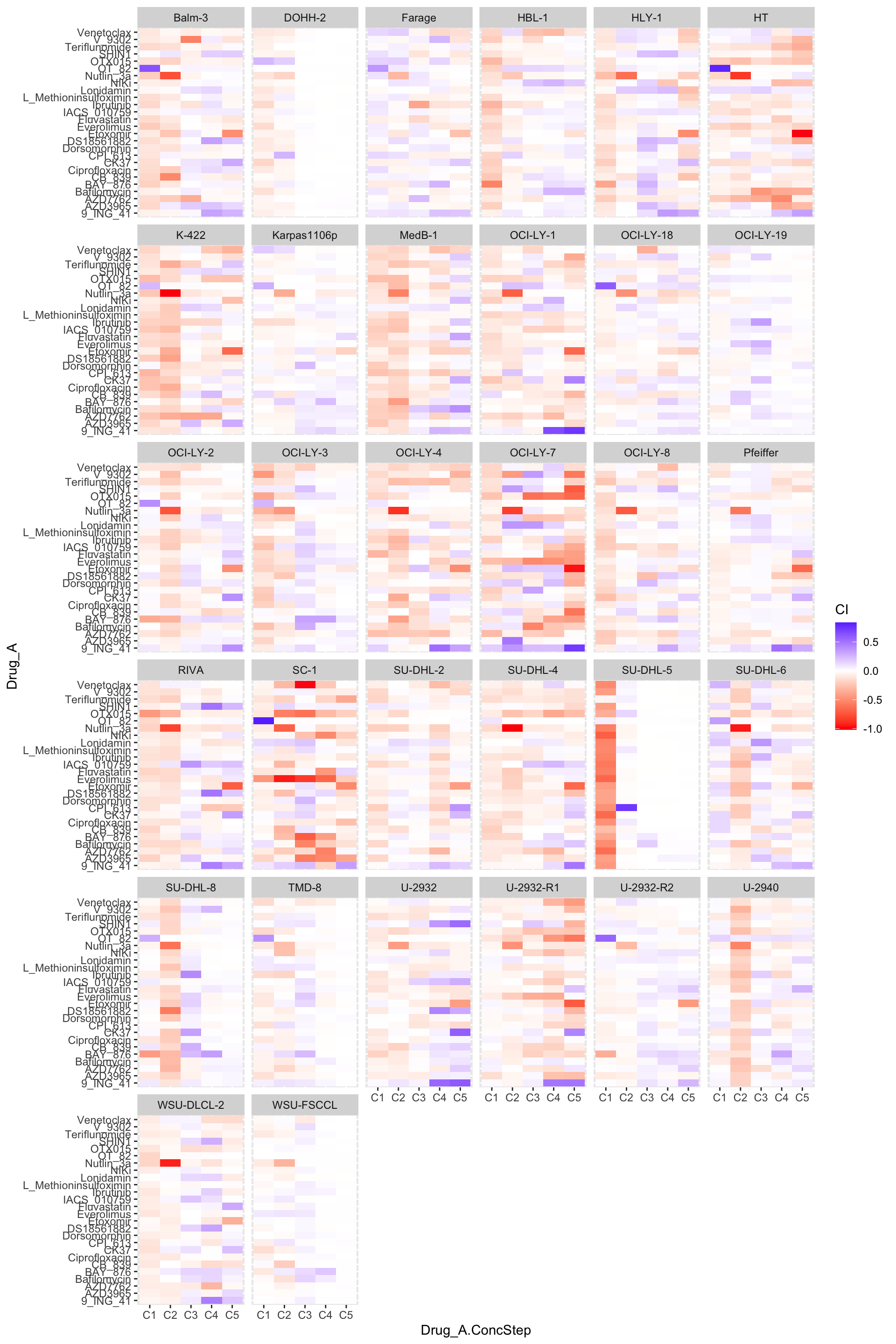

Summarise CI

Calculate synergistic and antagonistic effect separately, using a similar way as bayesyngergy package

sumSyn <- function(viabExp, viabObs) {
  tab <- tibble(viabExp=viabExp, viabObs = viabObs) %>%
    mutate(syn = min(0, viabObs - viabExp),
           anta = max(0, viabObs - viabExp))
  return(tibble(syn = sum(tab$syn), anta = sum(tab$anta)))
}

ciTabSum <- group_by(synTab, Name, Drug_A) %>% nest() %>%
  mutate(res = map(data, ~sumSyn(.$viabExp, .$viabObs))) %>%
  unnest(res) %>% select(-data)

Visualization of synergistic and antagoistic effect

Scatter plot

Top 5% synergistics or antagonistic effect are labelled.

plotSynScatter(ciTabSum, 0.05)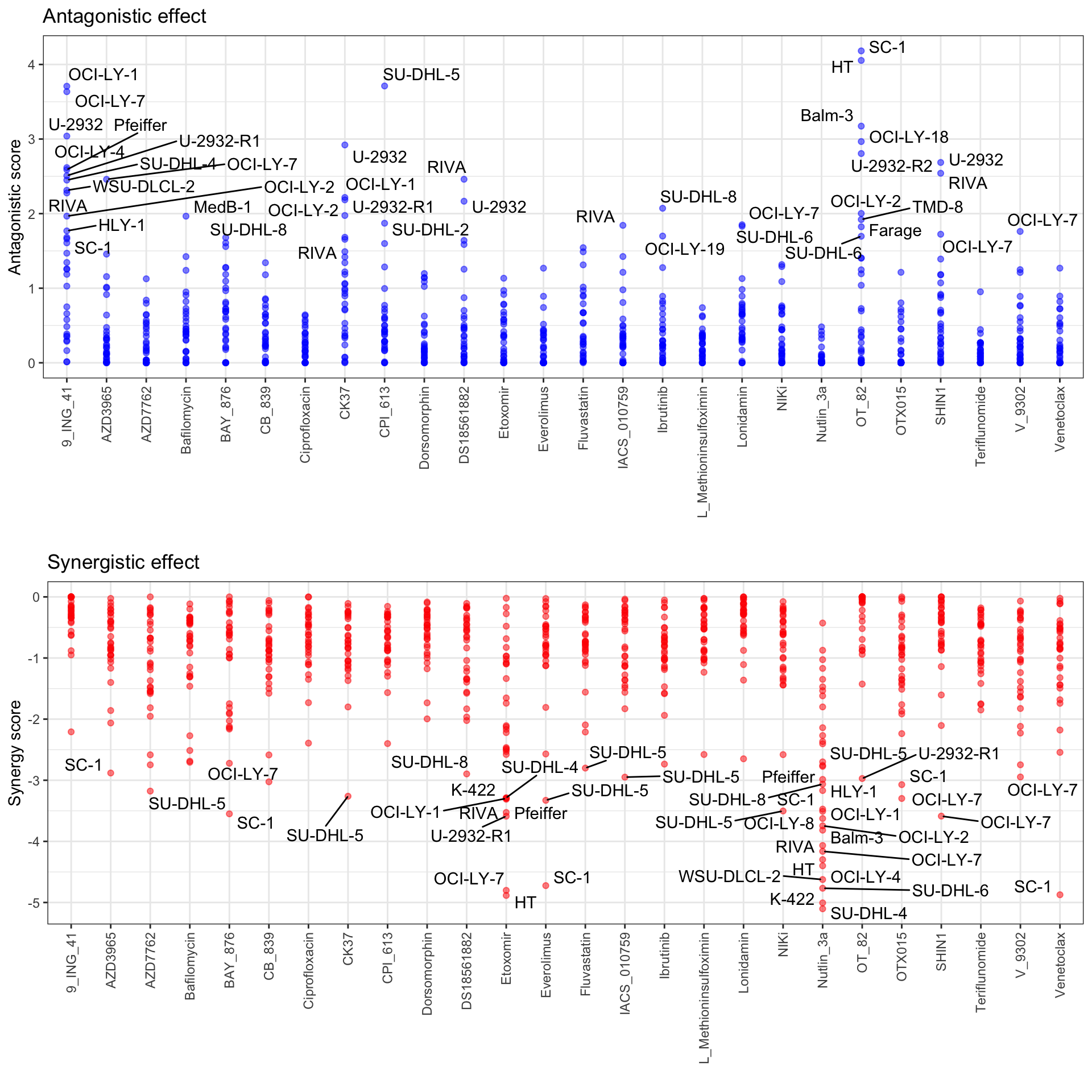

Matrix visualization

plotSynMatrix(ciTabSum, 0.1, 0.2)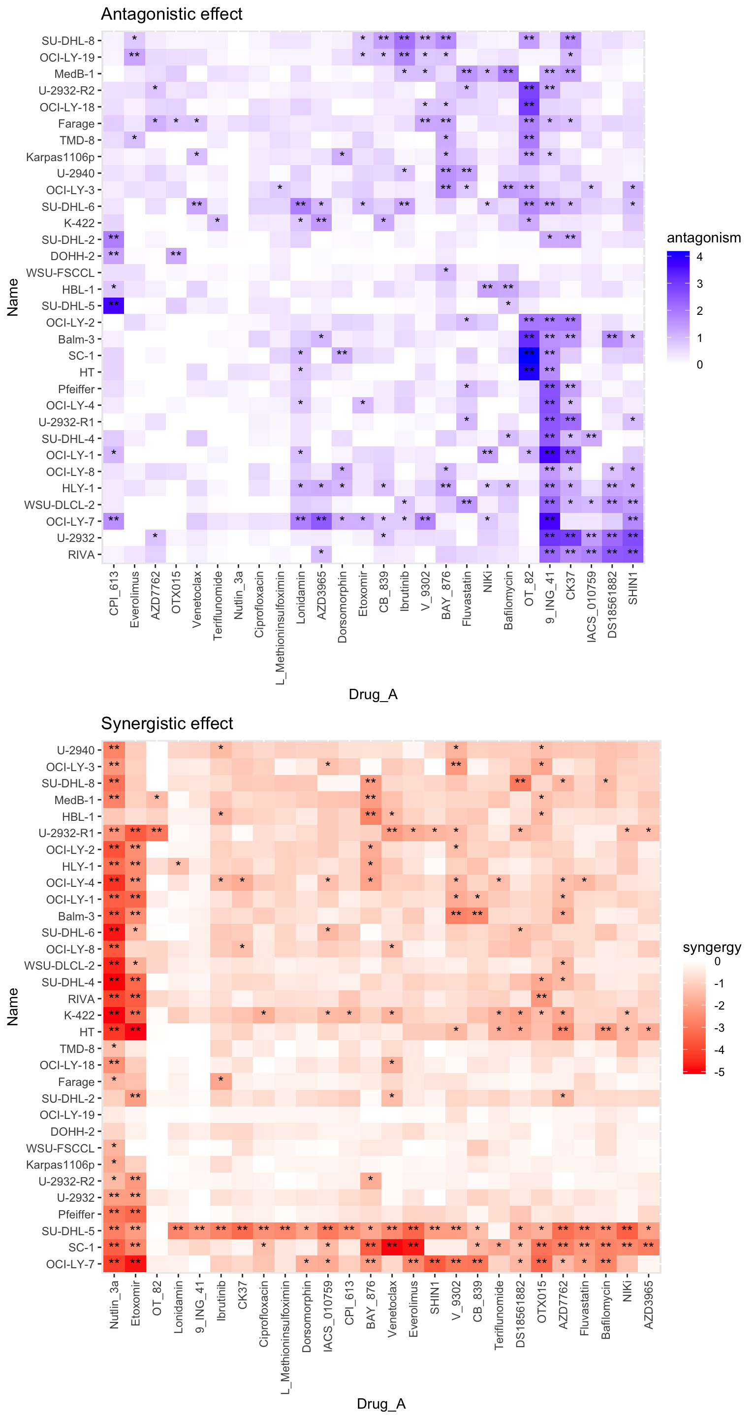

Top 10% synergistic/antagonistic effect are marked as ** and top 20% are marked as *

Correlate summarised CI to the single angent response of CHP_Pola

Add single agent CHP_Pola

polaTab <- screenData %>% filter(Drug_A == "DMSO", Drug_B == "CHP_Pola",!ifEdge) %>%
  group_by(Name) %>% summarise(viabPola = mean(normVal))

Test for correlation

testTab <- left_join(ciTabSum, polaTab, by = "Name") %>%
  pivot_longer(c("viabPola"), names_to = "Drug_B", values_to = "viab") %>%
  pivot_longer(c("syn","anta"), names_to = "effect", values_to = "score")

resTab <- group_by(testTab, Drug_A, Drug_B, effect) %>% nest() %>%
  mutate(m=map(data, ~cor.test(~score+viab,.))) %>%
  mutate(res = map(m, broom::tidy)) %>%
  unnest(res) %>%
  select(Drug_A, Drug_B, estimate, p.value, effect) %>%
  ungroup() %>% group_by(effect) %>%
  mutate(p.adj = p.adjust(p.value, method = "BH")) %>%
  arrange(p.value)

Correlation with synergistic

resTab.syn <- filter(resTab, p.adj <0.1, effect == "syn")
pList <- lapply(seq(nrow(resTab.syn)), function(i) {
  rec <- resTab.syn[i,]
  plotTab <- filter(testTab, Drug_A == rec$Drug_A, Drug_B==rec$Drug_B, effect == rec$effect)
  ggplot(plotTab, aes(x=viab, y=score, label = Name)) +
    geom_point(aes(col=Name)) +
    geom_smooth(method = "lm",se=FALSE) +
    ggrepel::geom_text_repel() +
    theme(legend.position = "none") +
    xlab(rec$Drug_B) + ylab("average CI") +
    ggtitle(sprintf("%s\n(p=%s, coef=%s)",rec$Drug_A, formatC(rec$p.value, digits = 2),formatC(rec$estimate, digits = 1)))
})
cowplot::plot_grid(plotlist=pList)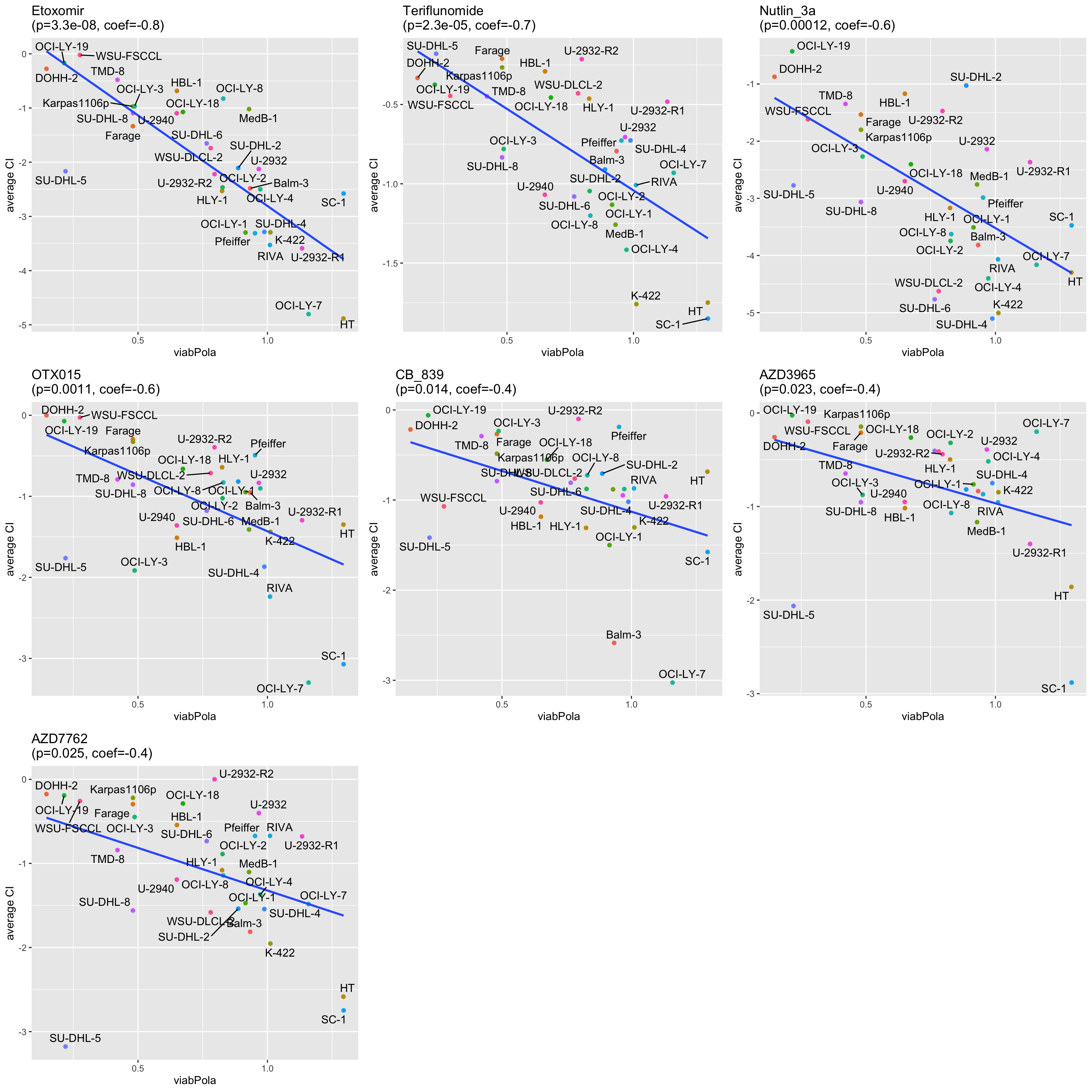

Correlation with antagonistic

resTab.anta <- filter(resTab, p.adj <0.1, effect == "anta")
pList <- lapply(seq(nrow(resTab.anta)), function(i) {
  rec <- resTab.anta[i,]
  plotTab <- filter(testTab, Drug_A == rec$Drug_A, Drug_B==rec$Drug_B, effect == rec$effect)
  ggplot(plotTab, aes(x=viab, y=score, label = Name)) +
    geom_point(aes(col=Name)) +
    geom_smooth(method = "lm",se=FALSE) +
    ggrepel::geom_text_repel() +
    theme(legend.position = "none") +
    xlab(rec$Drug_B) + ylab("average CI") +
    ggtitle(sprintf("%s\n(p=%s, coef=%s)",rec$Drug_A, formatC(rec$p.value, digits = 2),formatC(rec$estimate, digits = 1)))
})
cowplot::plot_grid(plotlist=pList)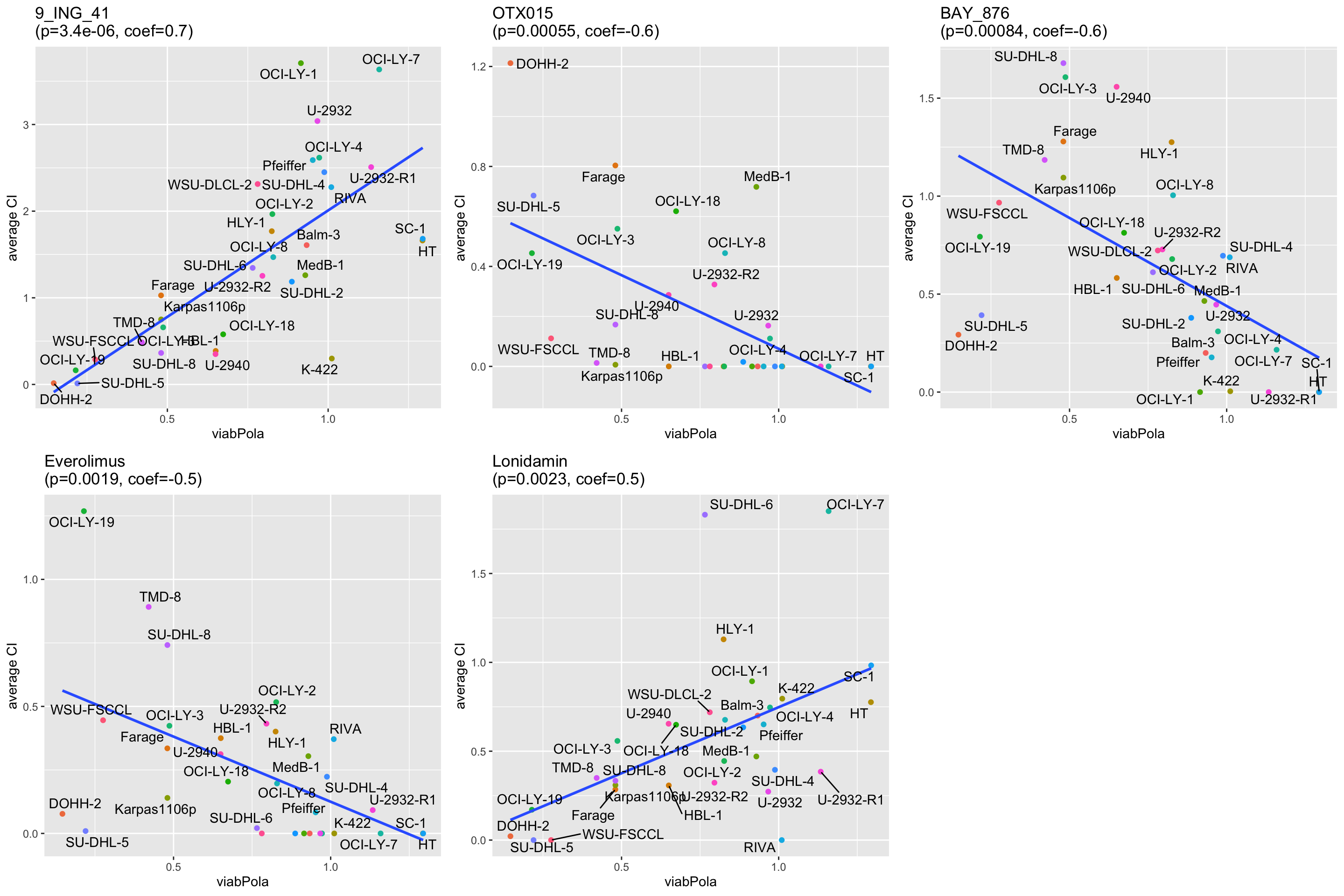

Plot combination curve for each drug, drug are ranked based on the sigificance correlation, cell lines are ranked based on CI

drugs <- unique(resTab$Drug_A)

pList <- lapply(drugs, function(eachDrug) {
  ciRank <- filter(ciTabSum, Drug_A==eachDrug) %>%
    arrange(syn)
  plotTab <- filter(synTab, Drug_A == eachDrug) %>%
    select(Name, Drug_A, Drug_A.ConcStep, viabA, viabB, viabExp, viabObs) %>%
    pivot_longer(-c("Name","Drug_A","Drug_A.ConcStep"), names_to = "type", values_to = "viab") %>%
    mutate(Name = factor(Name, levels = ciRank$Name)) %>%
    mutate(lineType = ifelse(type %in% c("viabA","viabB"), "single","combine"))
  
  ggplot(plotTab, aes(x=Drug_A.ConcStep, y=viab, group=type)) +
    geom_line(aes(col = type, linetype = lineType)) +
    facet_wrap(~Name) +
    scale_linetype_manual(values = c(combine = "solid", `single` = "dotted"), name = "combination") +
    scale_color_manual(values =c(viabA = "orange", viabB="darkgreen",
                                 viabExp = "red", viabObs="blue"),
                       labels=c("drug_A only ","drug_B only","expected effect","observed effect"),
                       name = "treatment") + 
    ggtitle(eachDrug) +
    ylab("Viability") + xlab("Concentration step")
})
jyluMisc::makepdf(pList, "../docs/combo_effect.pdf",nrow = 1, ncol = 1, height = 10, width = 10)

combo_effect.pdf

Test for synergistic effect related to genomics

Preprocess genomics

load("../data/SVs_filtered.RData")

mutTab <- svTab %>% filter(Name %in% synTab$Name) %>%
  group_by(Name, Gene) %>% summarise(n = length(Name)) %>%
  arrange(desc(n))

#Get mutations occured at least in three cell lines
geneCount <- group_by(mutTab, Gene) %>% summarise(n=length(Name)) %>%
  filter(n>=3) %>% arrange(desc(n)) 

mutTab <- filter(mutTab, Gene %in% geneCount$Gene) %>%
  mutate(status =1) %>% select(Name, Gene, status) %>%
  pivot_wider(names_from = "Gene", values_from = "status") %>%
  mutate_all(replace_na,0) %>%
  pivot_longer(-Name, names_to = "Gene", values_to = "status")

T-test

testTab <- ciTabSum %>% full_join(mutTab, by = "Name") %>%
  pivot_longer(c("syn","anta"), names_to = "effect", values_to = "CI") %>%
  filter(!is.na(Gene),!is.na(CI), effect =="syn")

resTab <- group_by(testTab, Drug_A, Gene, effect) %>% nest() %>%
  mutate(m = map(data, ~t.test(CI ~ status,., var.equal=TRUE))) %>%
  mutate(res = map(m, broom::tidy)) %>%
  unnest(res) %>%
  select(Drug_A, Gene, effect, estimate, p.value) %>%
  arrange(p.value) %>% ungroup() %>%
  mutate(p.adj = p.adjust(p.value, method = "BH"))

resTab.sig <- filter(resTab, p.value <= 0.05)

Boxplots for associations passed p-value <= 0.05

pList <- lapply(seq(nrow(resTab.sig)), function(i) {
  rec <- resTab.sig[i,]
  plotTab <- filter(testTab, Drug_A == rec$Drug_A, Gene == rec$Gene, effect == rec$effect) %>%
    mutate(status = factor(status))
  ggplot(plotTab, aes(x=status, y=CI)) +
    geom_boxplot(aes(fill = status)) +
    geom_point() +
    ggtitle(sprintf("%s ~ %s (p=%s)",rec$Drug_A, rec$Gene, formatC(rec$p.value, digits = 2))) +
    xlab(rec$Gene) +
    theme_bw() +
    theme(legend.position = "none")
})

cowplot::plot_grid(plotlist = pList, ncol=4)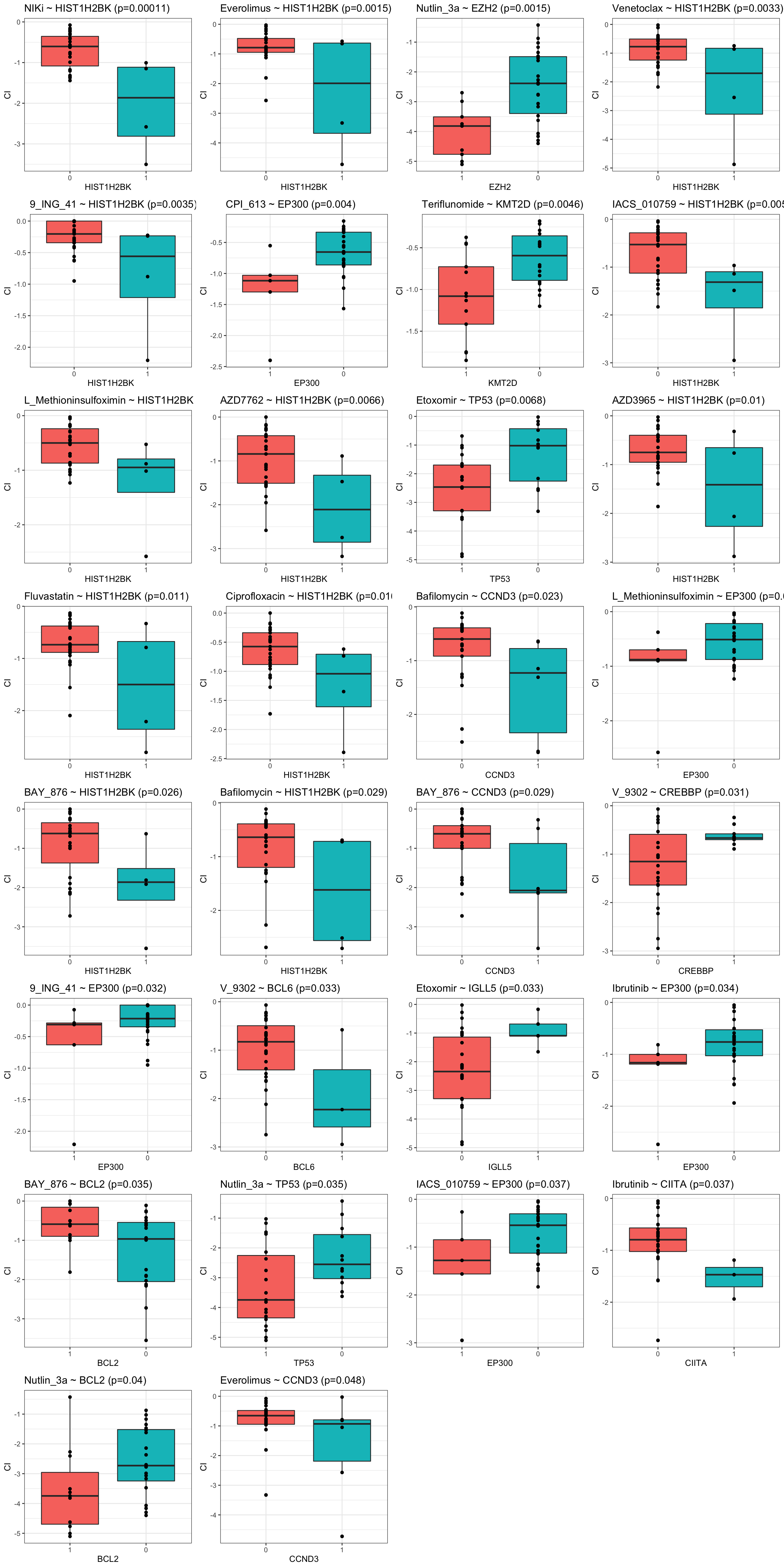

Heatmap

library(pheatmap)
ciTab <- testTab %>% 
  filter(Gene %in% resTab.sig$Gene, Drug_A %in% resTab.sig$Drug_A)

ciMat <- distinct(ciTab, Name, Drug_A, CI) %>%
  pivot_wider(names_from = "Name", values_from = "CI") %>%
  column_to_rownames("Drug_A") %>% as.matrix()

colAnno <- ciTab %>% ungroup() %>% distinct(Name, Gene, status) %>%
  mutate(status = as.character(status)) %>%
  pivot_wider(names_from = "Gene", values_from = "status") %>%
  column_to_rownames("Name")
annoColor <- lapply(colnames(colAnno), function(x) {c("1"="black","0"="white")})
names(annoColor) <- colnames(colAnno)
pheatmap(ciMat, annotation_col = colAnno, annotation_colors = annoColor)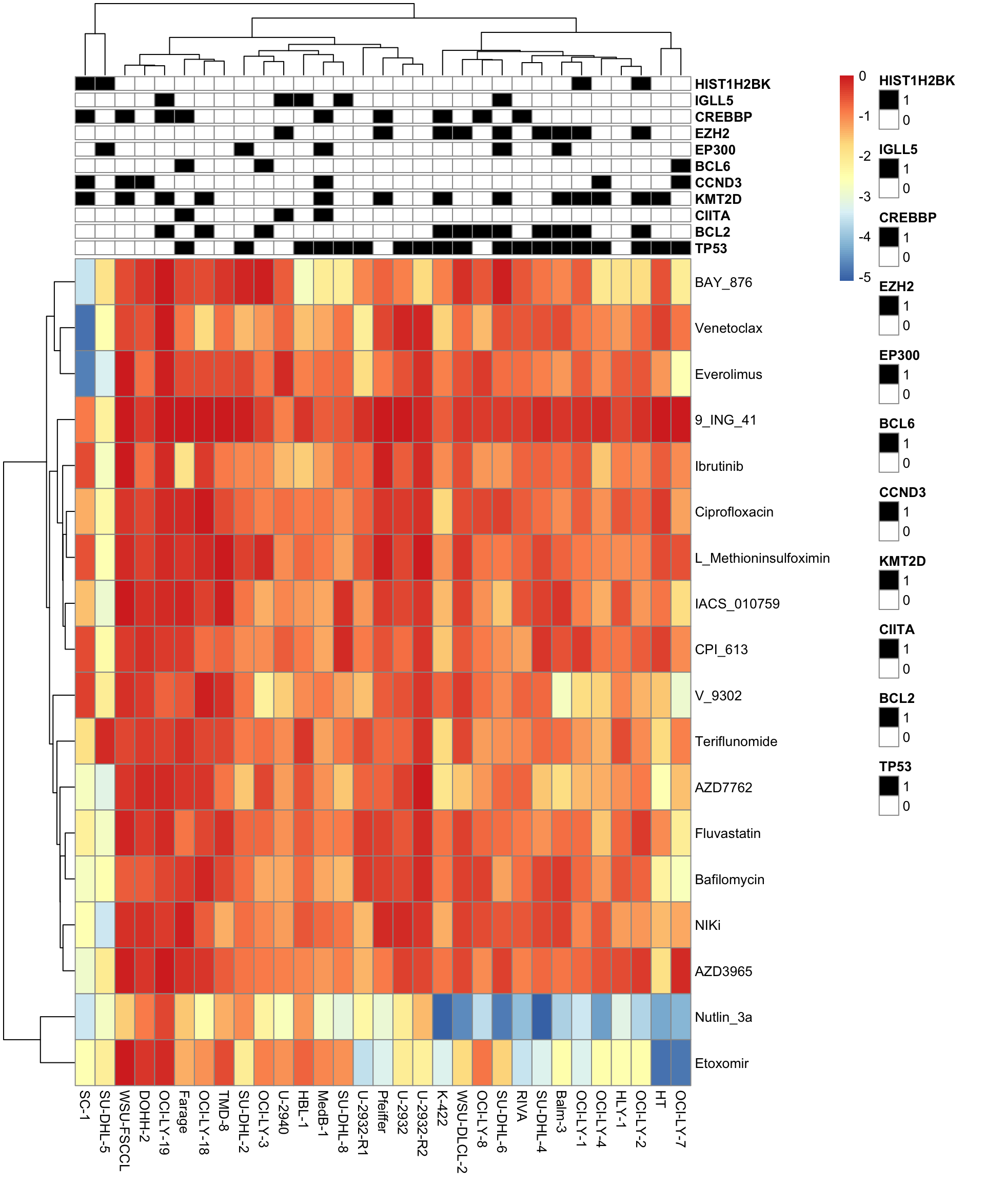

Does Etoxomir response/synergy associate with the expression of HSD17B4 or CPT1A?

Prepare Etoxomir response table

nonDLBCL <- c("Farage", "U-2940",   "MedB-1", "WSU-FSCCL", "SC-1", "Karpas-1106p")
etoTabCom <- ciTabSum %>% ungroup() %>% 
  filter(Drug_A == "Etoxomir") %>% select(Name, syn)
etoTabSingle <- drugATab %>% filter(Drug_A=="Etoxomir") %>%
  group_by(Name) %>% summarise(viab = mean(viabA))
etoTab <- left_join(etoTabCom, etoTabSingle) %>%
  pivot_longer(-Name, names_to = "type", values_to = "value") %>%
  filter(! Name %in% nonDLBCL ) #remove non-DLBCL cell lines

TP53 mutational status (fixed)

tp53MutTab <- mutTab %>% filter(Gene == "TP53") %>%
  mutate(status = ifelse(Name %in% c("Pfeiffer", "OCI-LY-8"),1,status)) %>%
  mutate(TP53 = ifelse(status ==1, "Mut", "WT")) %>%
  select(Name, TP53)

etoTab <- left_join(etoTab, tp53MutTab)

RNAseq expression

Preprocessing

library(matrixStats)
load("../data/DepMap_GEXwide.RData")
exprMat <- t(DepMap_GEXwide)
exprMat <- exprMat[,colnames(exprMat) %in% etoTab$Name]

# Remove low count genes
#exprMat <- exprMat[rowMedians(exprMat) >0,]

#vstObj <- vsn::vsnMatrix(exprMat)
#exprMat <- vsn::predict(vstObj, exprMat)

Select two interested genes

exprTab <- exprMat[c("HSD17B4","CPT1A"),] %>%
  as_tibble(rownames = "Gene") %>%
  pivot_longer(-Gene,names_to = "Name",values_to = "expr")

Correlation test

testTab <- left_join(exprTab, etoTab, by = "Name")
resTab <- group_by(testTab, Gene, type) %>% nest() %>%
  mutate(m=map(data,~cor.test(~expr+value,.))) %>%
  mutate(res = map(m, broom::tidy)) %>%
  unnest(res) %>%
  select(Gene, type, p.value, estimate)
resTab

# A tibble: 4 × 4
# Groups:   Gene, type [4]
  Gene    type  p.value estimate
  <chr>   <chr>   <dbl>    <dbl>
1 HSD17B4 syn   0.102    -0.474 
2 HSD17B4 viab  0.840    -0.0621
3 CPT1A   syn   0.00311  -0.751 
4 CPT1A   viab  0.413    -0.249 

“Syn” indicates synergy (CI values), “viab” indicates single agent response

Correlation plot

ggplot(testTab, aes(x=expr, y = value)) +
  ggrepel::geom_text_repel(aes(label = Name)) +
  geom_point(aes(col = TP53)) +
  geom_smooth(method = "lm") +
  facet_wrap(~Gene + type, scale = "free")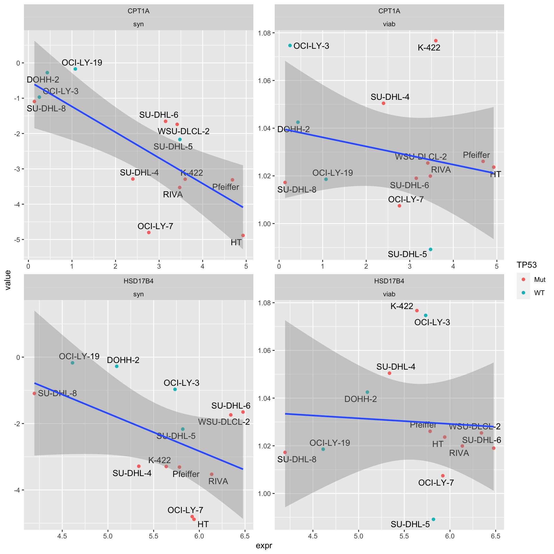

Proteom expression (SMART-CARE)

Preprocessing

library(SummarizedExperiment)
protData <- readRDS("../data/SC005_SummarizedExperiment_proteomics.RDS")
#select baseline samples
protData <- protData[rowData(protData)$Gene_name %in% c("HSD17B4","CPT1A"), protData$cell.line %in% etoTab$Name & protData$condition == "U"]
exprMat <- assay(protData)
rownames(exprMat) <- rowData(protData)$Gene_name

Select two interested genes

protTab <- exprMat[c("HSD17B4","CPT1A"),] %>%
  as_tibble(rownames = "Gene") %>%
  pivot_longer(-Gene,names_to = "smp",values_to = "expr") %>%
  mutate(Name = protData[,smp]$cell.line) %>%
  group_by(Gene,Name) %>%
  summarise(expr = mean(expr, na.rm=TRUE)) %>% ungroup() %>%
  filter(!is.na(expr))

Correlation test

testTab <- left_join(protTab, etoTab, by = "Name")
resTab <- group_by(testTab, Gene, type) %>% nest() %>%
  mutate(m=map(data,~cor.test(~expr+value,., use= "pairwise.complete.obs"))) %>%
  mutate(res = map(m, broom::tidy)) %>%
  unnest(res) %>%
  select(Gene, type, p.value, estimate)
resTab

# A tibble: 4 × 4
# Groups:   Gene, type [4]
  Gene    type  p.value  estimate
  <chr>   <chr>   <dbl>     <dbl>
1 CPT1A   syn    0.678  -0.150   
2 CPT1A   viab   0.999   0.000656
3 HSD17B4 syn    0.0235 -0.645   
4 HSD17B4 viab   0.471   0.230   

“Syn” indicates synergy (CI values), “viab” indicates single agent response

Correlation plot

ggplot(testTab, aes(x=expr, y = value)) +
  ggrepel::geom_text_repel(aes(label = Name)) +
  geom_point(aes(col = TP53)) +
  geom_smooth(method = "lm") +
  facet_wrap(~Gene + type, scale = "free")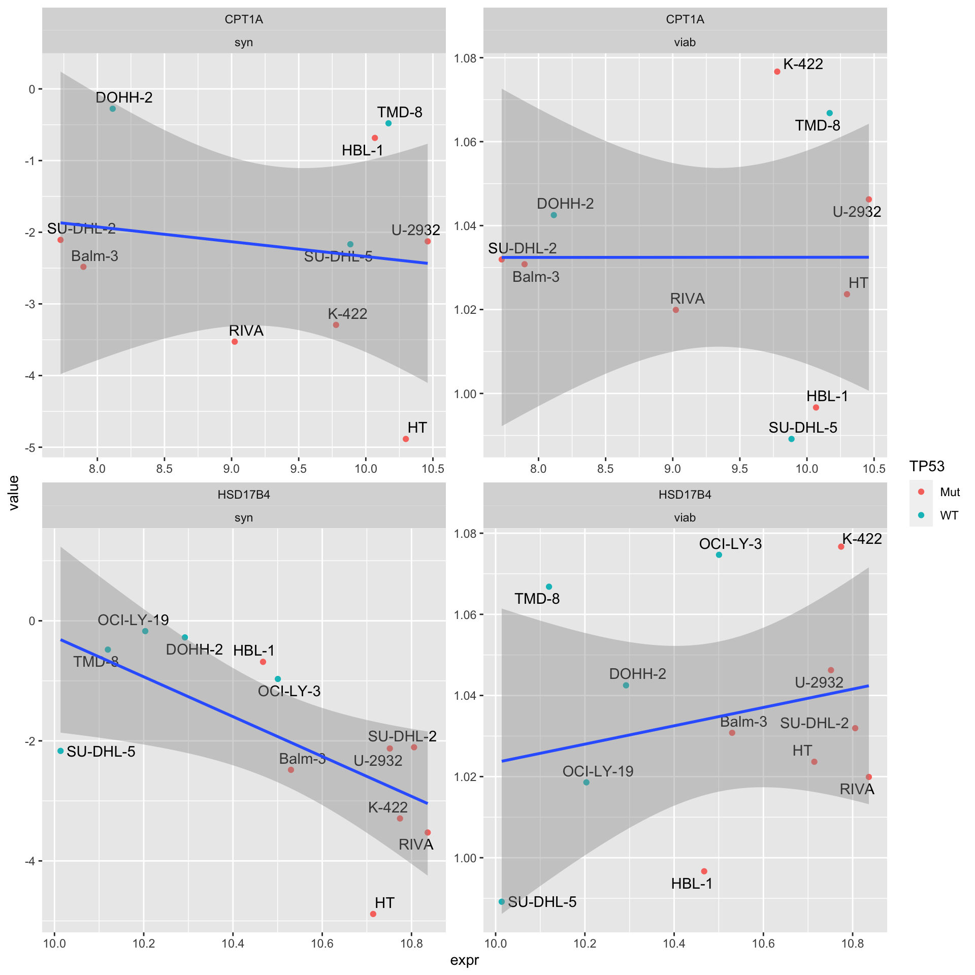

Proteom expression (EMBL)

Preprocessing

load("../data/ProtWide.RData")
ProtWide <- ProtWide[,colnames(ProtWide) %in% etoTab$Name]
exprMat <- ProtWide

Select two interested genes

protTab1 <- exprMat[c("HSD17B4","CPT1A"),] %>%
  as_tibble(rownames = "Gene") %>%
  pivot_longer(-Gene,names_to = "Name",values_to = "expr")

Correlation test

testTab <- left_join(protTab1, etoTab, by = "Name")
resTab <- group_by(testTab, Gene, type) %>% nest() %>%
  mutate(m=map(data,~cor.test(~expr+value,., use= "pairwise.complete.obs"))) %>%
  mutate(res = map(m, broom::tidy)) %>%
  unnest(res) %>%
  select(Gene, type, p.value, estimate)
resTab

# A tibble: 4 × 4
# Groups:   Gene, type [4]
  Gene    type  p.value estimate
  <chr>   <chr>   <dbl>    <dbl>
1 HSD17B4 syn    0.0617  -0.372 
2 HSD17B4 viab   0.561   -0.120 
3 CPT1A   syn    0.105   -0.326 
4 CPT1A   viab   0.942   -0.0150

“Syn” indicates synergy (CI values), “viab” indicates single agent response

Correlation plot

ggplot(testTab, aes(x=expr, y = value)) +
  ggrepel::geom_text_repel(aes(label = Name)) +
  geom_point(aes(col = TP53)) +
  geom_smooth(method = "lm") +
  facet_wrap(~Gene + type, scale = "free")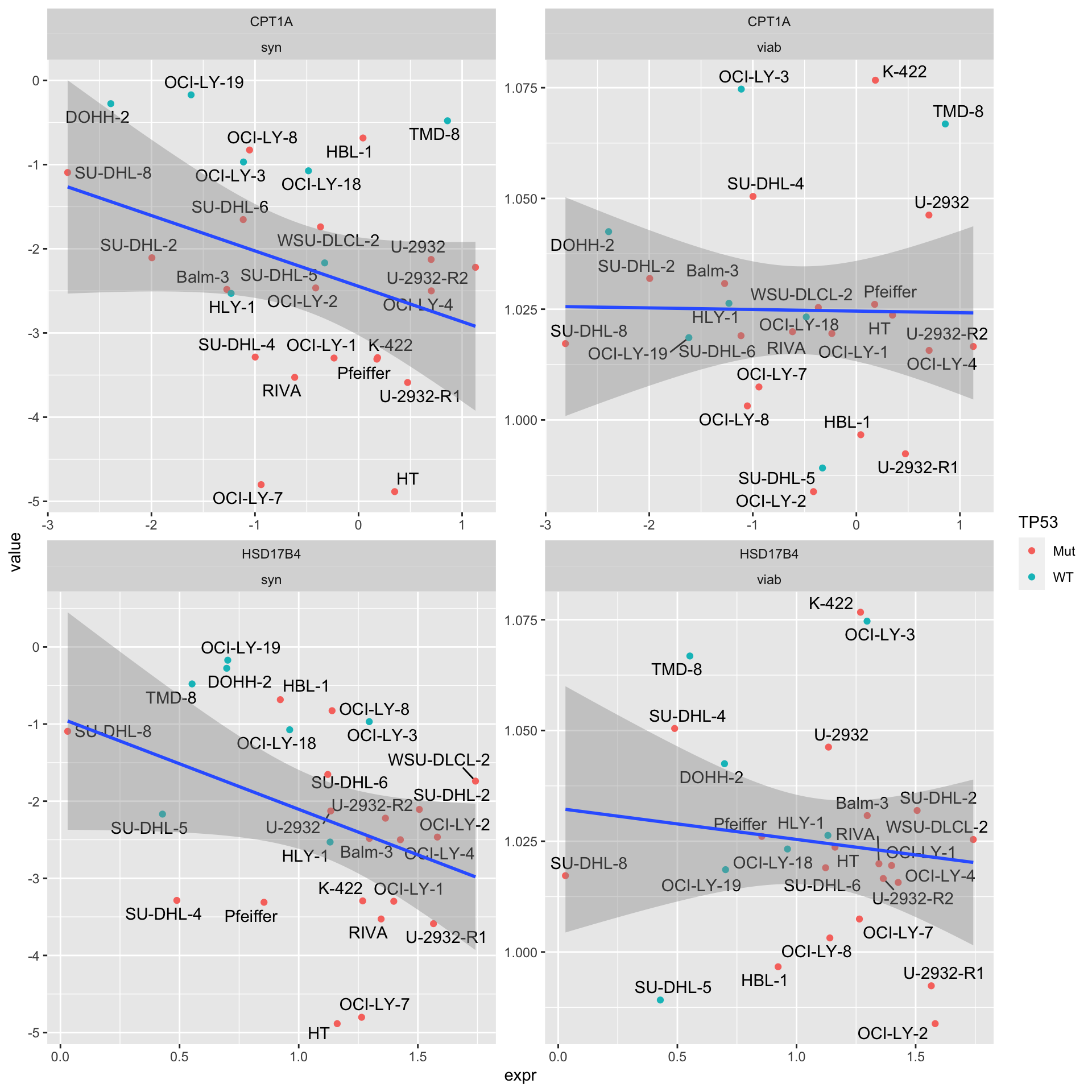

Does Etoxomir response/synergy associate with the abundance of any metabolites?

Preprocessing

metaData <- readRDS("../data/SC005_SummarizedExperiment_metabolomics.RDS")
metaData <- metaData[metaData$condition == "U",metaData$cell.line %in% etoTab$Name]
metaMat <- assay(metaData)

metaMatNorm <- PhosR::medianScaling(metaMat, scale = FALSE)
#vsnFit <- vsn::vsnMatrix(metaMat)
#metaMatNorm <- metaMat
#boxplot(metaMatNorm)
metaNorm <- metaData
assay(metaNorm) <- metaMatNorm
assayNames(metaNorm) <- "norm"
exprMat <- assay(metaNorm)

Select two interested genes

metaTab <- exprMat %>%
  as_tibble(rownames = "Metabolite") %>%
  pivot_longer(-Metabolite,names_to = "smp",values_to = "expr") %>%
  mutate(Name = metaNorm[,smp]$cell.line) %>%
  group_by(Metabolite,Name) %>%
  summarise(expr = mean(expr, na.rm=TRUE)) %>% ungroup() %>%
  filter(!is.na(expr))

Correlation test

testTab <- left_join(metaTab, etoTab, by = "Name")
resTab <- group_by(testTab, Metabolite, type) %>% nest() %>%
  mutate(m=map(data,~cor.test(~expr+value,., use= "pairwise.complete.obs"))) %>%
  mutate(res = map(m, broom::tidy)) %>%
  unnest(res) %>%
  select(Metabolite, type, p.value, estimate) %>%
  arrange(p.value)
resTab

# A tibble: 286 × 4
# Groups:   Metabolite, type [286]
   Metabolite          type  p.value estimate
   <chr>               <chr>   <dbl>    <dbl>
 1 Hex2Cer(d18:1/24:0) syn   0.00107    0.821
 2 HexCer(d18:2/16:0)  syn   0.0184    -0.664
 3 DG-O(16:0_18:1)     syn   0.0204    -0.656
 4 Cer(d18:2/24:1)     syn   0.0212    -0.653
 5 Hex2Cer(d18:1/26:1) syn   0.0229     0.647
 6 Betaine             syn   0.0244    -0.642
 7 HexCer(d18:2/24:0)  viab  0.0247    -0.641
 8 Hex2Cer(d18:1/24:1) syn   0.0280     0.630
 9 HexCer(d18:2/24:0)  syn   0.0285    -0.629
10 PC ae C34:1         syn   0.0313    -0.620
# … with 276 more rows
# ℹ Use `print(n = ...)` to see more rows

“Syn” indicates synergy (CI values), “viab” indicates single agent response

Correlation plot

ggplot(filter(testTab, Metabolite %in% resTab[1:9,]$Metabolite), aes(x=expr, y = value)) +
  ggrepel::geom_text_repel(aes(label = Name)) +
  geom_point(aes(col = TP53)) +
  geom_smooth(method = "lm") +
  facet_wrap(~Metabolite + type, scale = "free")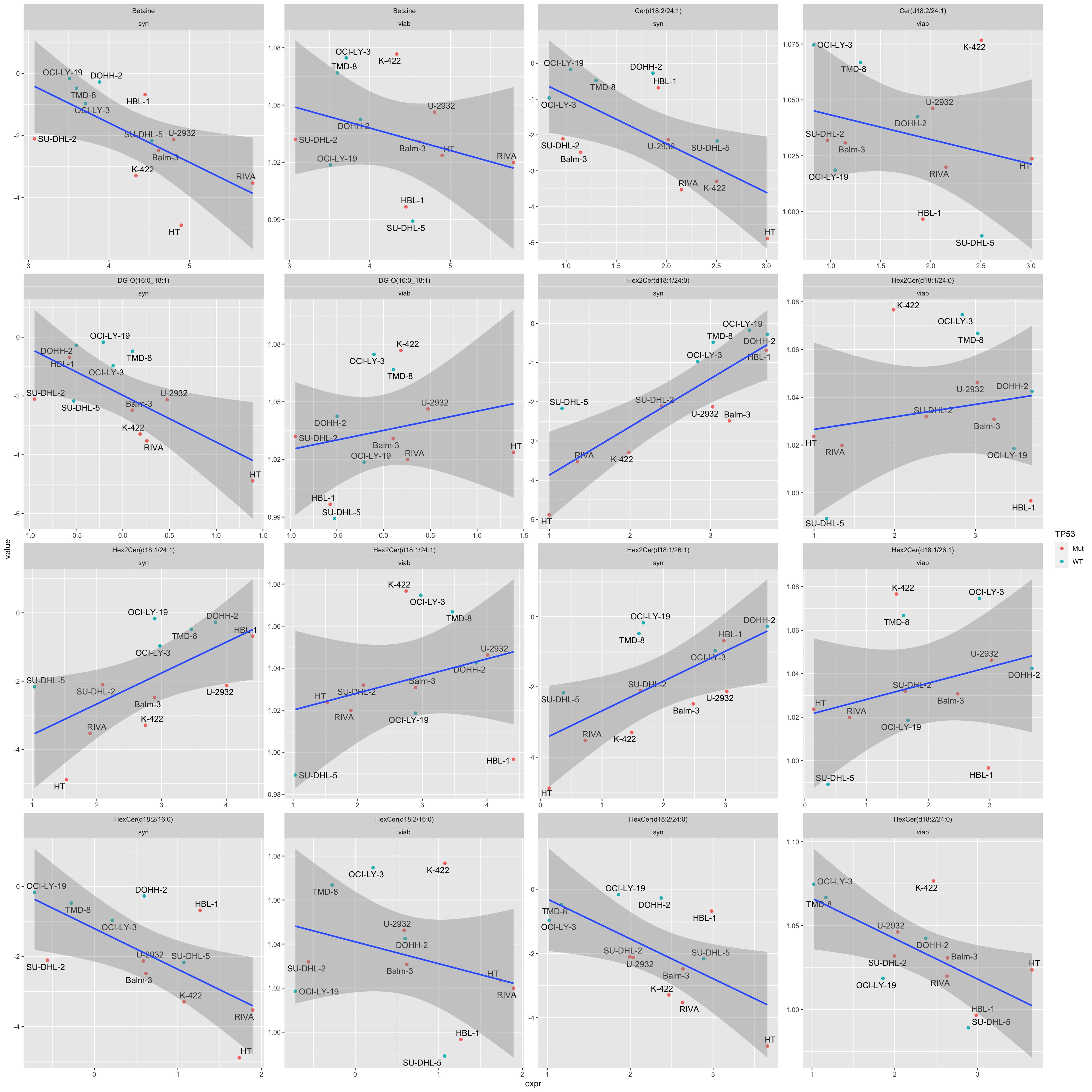

Correlation gene/protein expression of HSD17B4 and CPT1A with metabolites

exprTabAll <- bind_rows(mutate(exprTab, set = "RNA"),
                        mutate(protTab, set = "Protein_SMART"),
                        mutate(protTab1, set = "Protein_EMBL"))
testTab <- full_join(exprTabAll, dplyr::rename(metaTab, abundance = expr), by = "Name") %>%
  filter(!is.na(expr), !is.na(abundance)) %>%
  left_join(tp53MutTab)

resTab <- group_by(testTab, Gene, set, Metabolite) %>% nest() %>%
  mutate(m=map(data, ~cor.test(~expr+abundance,.))) %>%
  mutate(res = map(m, broom::tidy)) %>%
  unnest(res) %>%
  select(Gene, set, Metabolite, estimate, p.value) %>%
  arrange(p.value) %>% ungroup() %>%
  mutate(p.adj = p.adjust(p.value, method = "BH"))

Result table (FDR < 0.1)

resTab.sig <- filter(resTab, p.adj <= 0.1)
resTab.sig %>% mutate_if(is.numeric, formatC, digits=2) %>%
  DT::datatable()

Correlation plots of significant associations

pList <- lapply(seq(9), function(i) {
  rec <- resTab.sig[i,]
  plotTab <- testTab %>% filter(Gene == rec$Gene, set == rec$set, Metabolite == rec$Metabolite)
  ggplot(plotTab, aes(x=expr, y=abundance)) +
    geom_point(aes(col = TP53)) +
    geom_smooth(method = "lm") +
    ggrepel::geom_text_repel(aes(label = Name)) +
    ggtitle(sprintf("%s ~ %s\n(P=%s, %s)", rec$Metabolite, rec$Gene, formatC(rec$p.value, digits = 2), rec$set)) +
    theme_bw()
})
cowplot::plot_grid(plotlist = pList, ncol=3)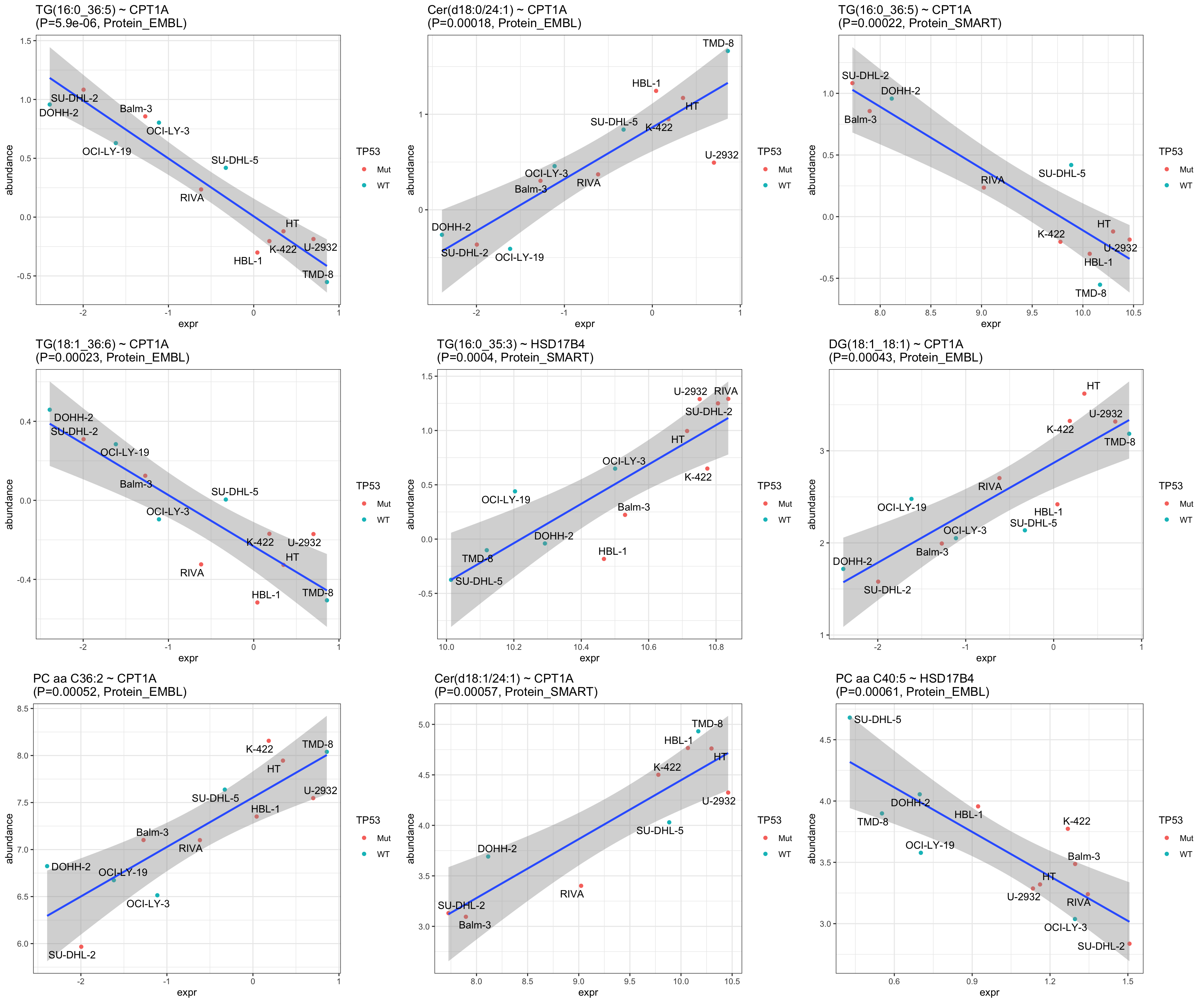

Session information

sessionInfo()

R version 4.2.0 (2022-04-22)
Platform: x86_64-apple-darwin17.0 (64-bit)
Running under: macOS Big Sur/Monterey 10.16

Matrix products: default
BLAS:   /Library/Frameworks/R.framework/Versions/4.2/Resources/lib/libRblas.0.dylib
LAPACK: /Library/Frameworks/R.framework/Versions/4.2/Resources/lib/libRlapack.dylib

locale:
[1] en_US.UTF-8/en_US.UTF-8/en_US.UTF-8/C/en_US.UTF-8/en_US.UTF-8

attached base packages:
[1] stats4    stats     graphics  grDevices utils     datasets  methods  
[8] base     

other attached packages:
 [1] SummarizedExperiment_1.26.1 Biobase_2.56.0             
 [3] GenomicRanges_1.48.0        GenomeInfoDb_1.32.2        
 [5] IRanges_2.30.0              S4Vectors_0.34.0           
 [7] BiocGenerics_0.42.0         MatrixGenerics_1.8.1       
 [9] matrixStats_0.62.0          pheatmap_1.0.12            
[11] gridExtra_2.3               forcats_0.5.1              
[13] stringr_1.4.0               dplyr_1.0.9                
[15] purrr_0.3.4                 readr_2.1.2                
[17] tidyr_1.2.0                 tibble_3.1.8               
[19] ggplot2_3.3.6               tidyverse_1.3.2            

loaded via a namespace (and not attached):
  [1] utf8_1.2.2             shinydashboard_0.7.2   tidyselect_1.1.2      
  [4] htmlwidgets_1.5.4      grid_4.2.0             BiocParallel_1.30.3   
  [7] maxstat_0.7-25         munsell_0.5.0          preprocessCore_1.58.0 
 [10] codetools_0.2-18       DT_0.23                withr_2.5.0           
 [13] colorspace_2.0-3       highr_0.9              knitr_1.39            
 [16] rstudioapi_0.13        ggsignif_0.6.3         labeling_0.4.2        
 [19] git2r_0.30.1           slam_0.1-50            GenomeInfoDbData_1.2.8
 [22] KMsurv_0.1-5           farver_2.1.1           rprojroot_2.0.3       
 [25] coda_0.19-4            vctrs_0.4.1            generics_0.1.3        
 [28] TH.data_1.1-1          xfun_0.31              sets_1.0-21           
 [31] R6_2.5.1               bitops_1.0-7           cachem_1.0.6          
 [34] reshape_0.8.9          fgsea_1.22.0           DelayedArray_0.22.0   
 [37] assertthat_0.2.1       promises_1.2.0.1       scales_1.2.0          
 [40] multcomp_1.4-19        googlesheets4_1.0.0    gtable_0.3.0          
 [43] sandwich_3.0-2         workflowr_1.7.0        rlang_1.0.4           
 [46] GlobalOptions_0.1.2    splines_4.2.0          rstatix_0.7.0         
 [49] gargle_1.2.0           broom_1.0.0            reshape2_1.4.4        
 [52] yaml_2.3.5             abind_1.4-5            modelr_0.1.8          
 [55] crosstalk_1.2.0        backports_1.4.1        httpuv_1.6.5          
 [58] tools_4.2.0            relations_0.6-12       statnet.common_4.6.0  
 [61] ellipsis_0.3.2         gplots_3.1.3           jquerylib_0.1.4       
 [64] RColorBrewer_1.1-3     ggdendro_0.1.23        proxy_0.4-27          
 [67] Rcpp_1.0.9             plyr_1.8.7             visNetwork_2.1.0      
 [70] zlibbioc_1.42.0        RCurl_1.98-1.7         ggpubr_0.4.0          
 [73] viridis_0.6.2          cowplot_1.1.1          zoo_1.8-10            
 [76] haven_2.5.0            ggrepel_0.9.1          cluster_2.1.3         
 [79] exactRankTests_0.8-35  fs_1.5.2               magrittr_2.0.3        
 [82] data.table_1.14.2      PhosR_1.6.0            circlize_0.4.15       
 [85] reprex_2.0.1           survminer_0.4.9        pcaMethods_1.88.0     
 [88] googledrive_2.0.0      mvtnorm_1.1-3          hms_1.1.1             
 [91] shinyjs_2.1.0          mime_0.12              evaluate_0.15         
 [94] xtable_1.8-4           readxl_1.4.0           shape_1.4.6           
 [97] compiler_4.2.0         KernSmooth_2.23-20     crayon_1.5.1          
[100] htmltools_0.5.3        mgcv_1.8-40            later_1.3.0           
[103] tzdb_0.3.0             lubridate_1.8.0        DBI_1.1.3             
[106] dbplyr_2.2.1           MASS_7.3-58            jyluMisc_0.1.5        
[109] Matrix_1.4-1           car_3.1-0              cli_3.3.0             
[112] marray_1.74.0          parallel_4.2.0         igraph_1.3.4          
[115] pkgconfig_2.0.3        km.ci_0.5-6            piano_2.12.0          
[118] xml2_1.3.3             bslib_0.4.0            ruv_0.9.7.1           
[121] XVector_0.36.0         drc_3.0-1              rvest_1.0.2           
[124] digest_0.6.29          rmarkdown_2.14         cellranger_1.1.0      
[127] fastmatch_1.1-3        survMisc_0.5.6         dendextend_1.16.0     
[130] shiny_1.7.2            gtools_3.9.3           lifecycle_1.0.1       
[133] nlme_3.1-158           jsonlite_1.8.0         carData_3.0-5         
[136] network_1.17.2         viridisLite_0.4.0      limma_3.52.2          
[139] fansi_1.0.3            pillar_1.8.0           lattice_0.20-45       
[142] GGally_2.1.2           fastmap_1.1.0          httr_1.4.3            
[145] plotrix_3.8-2          survival_3.3-1         glue_1.6.2            
[148] class_7.3-20           stringi_1.7.8          sass_0.4.2            
[151] caTools_1.18.2         e1071_1.7-11