Last updated: 2023-06-16

Checks: 5 1

Knit directory: combiDLBCL/analysis/

This reproducible R Markdown analysis was created with workflowr (version 1.7.0). The Checks tab describes the reproducibility checks that were applied when the results were created. The Past versions tab lists the development history.

Environment: empty

Great job! The global environment was empty. Objects defined in the global environment can affect the analysis in your R Markdown file in unknown ways. For reproduciblity it’s best to always run the code in an empty environment.

Seed: set.seed(20220425)

The command set.seed(20220425) was run prior to running the code in the R Markdown file. Setting a seed ensures that any results that rely on randomness, e.g. subsampling or permutations, are reproducible.

Session information: recorded

Great job! Recording the operating system, R version, and package versions is critical for reproducibility.

Cache: none

Nice! There were no cached chunks for this analysis, so you can be confident that you successfully produced the results during this run.

File paths: relative

Great job! Using relative paths to the files within your workflowr project makes it easier to run your code on other machines.

Repository version: no version control

Tracking code development and connecting the code version to the results is critical for reproducibility. To start using Git, open the Terminal and type git init in your project directory.

This project is not being versioned with Git. To obtain the full reproducibility benefits of using workflowr, please see ?wflow_start.

Load libraries and datasets

Calculate CI for the combination of bases and combi drugs

screenSub <- screenData %>% 
  mutate(Name = cellLine, normVal = normVal.cor) %>%
  filter(!ifRemove)

Get combination effect

comTab <- filter(screenSub, Drug_A !="DMSO", Drug_B != "DMSO") %>%
  select(Name, Drug_A, Drug_A.Conc, Drug_B, Drug_B.Conc, normVal) %>%
  dplyr::rename(viabObs = normVal) %>%
  distinct(Name, Drug_A, Drug_A.Conc, Drug_B, Drug_B.Conc, .keep_all = TRUE)

drugATab <- filter(screenSub, Drug_A != "DMSO", Drug_B == "DMSO") %>%
  select(Name, Drug_A, Drug_A.Conc, normVal, Drug_A.ConcStep) %>%
  dplyr::rename(viabA = normVal) %>%
  distinct(Name, Drug_A, Drug_A.Conc, .keep_all = TRUE)

drugBTab <- filter(screenSub, Drug_A == "DMSO", Drug_B != "DMSO") %>%
  select(Name, Drug_B, Drug_B.Conc, normVal, Drug_B.ConcStep) %>%
  dplyr::rename(viabB = normVal) %>%
  distinct(Name,Drug_B, Drug_B.Conc, .keep_all = TRUE)

synTab <- comTab %>% left_join(drugATab, by =c("Name","Drug_A","Drug_A.Conc")) %>%
  left_join(drugBTab, by = c("Name","Drug_B","Drug_B.Conc")) %>%
  mutate(viabExp = viabA*viabB) %>%
  mutate(CI = viabObs-viabExp,
         logCI = log10(viabObs/viabExp))

Save CI table for shiny app

save(synTab, file = "../shiny/combiDLBCL/synTab_AA2022.RData")

Visualize CI for each drug and concentration

pList <- lapply(unique(synTab$Drug_A), function(drugA) {
  plotTab <- filter(synTab, Drug_A == drugA)
  
  ggplot(plotTab, aes(x=Drug_B.ConcStep, y=Drug_B, fill = CI)) +
  geom_tile() +
  facet_wrap(~Name, ncol=5) +
  scale_fill_gradient2(low ="red",high="blue",mid="white") +
    ggtitle(drugA)
  
})
names(pList) <- unique(synTab$Drug_A)

jyluMisc::makepdf(pList, "../docs/CI_heatmap_AAscreen2023.pdf", height = 30, width = 10, ncol = 1, nrow = 1)

CI_heatmap_AAscreen2023.pdf

Summarise CI

Calculate synergistic and antagonistic effect separately, using a similar way as bayesyngergy package

sumSyn <- function(viabExp, viabObs) {
  tab <- tibble(viabExp=viabExp, viabObs = viabObs) %>%
    mutate(syn = min(0, viabObs - viabExp),
           anta = max(0, viabObs - viabExp))
  return(tibble(syn = sum(tab$syn,na.rm = TRUE), anta = sum(tab$anta,na.rm = TRUE)))
}

ciTabSum <- group_by(synTab, Name, Drug_A, Drug_B) %>% nest() %>%
  mutate(res = map(data, ~sumSyn(.$viabExp, .$viabObs))) %>%
  unnest(res) %>% select(-data)

Visualization of synergistic and antagoistic effect

plotSynScatter <- function(plotTab, labelPercent = 0.05) {
  
  synCut <-  quantile(plotTab$syn, labelPercent)
  antaCut <- quantile(plotTab$anta, 1-labelPercent)
  
  plotTabSyn <- plotTab %>% mutate(labelText = ifelse(syn < synCut, Name,""), type = "Synergistic effect") %>%
    mutate(score = syn)
  plotTabAnta <- plotTab %>% mutate(labelText = ifelse(anta > antaCut, Name,""), type = "Antagonistic effect") %>%
    mutate(score = anta)
  plotComb <- bind_rows(plotTabSyn, plotTabAnta)
  
  p <- ggplot(plotComb, aes(x=Drug_B, y=score, label = labelText)) +
    geom_point(aes(col= type), alpha=0.5) + ggrepel::geom_text_repel(max.overlaps = Inf) +
    theme_bw() +
    theme(axis.text.x = element_text(angle = 90, hjust=1, vjust = 0.5)) +
    scale_color_manual(values = c("Synergistic effect" = "red", "Antagonistic effect" = "blue")) +
    #facet_wrap(~type, ncol=2)
    ggtitle(unique(plotComb$Drug_A)) + ylab("Combination Score") + xlab("") +
    theme(legend.position = "bottom")
  return(p)
}

Scatter plot

Top 5% synergistics or antagonistic effect are labelled.

pList <- lapply(unique(ciTabSum$Drug_A), function(drugA){
  plotTab <- filter(ciTabSum, Drug_A == drugA)
  plotSynScatter(plotTab,0.05)
})
jyluMisc::makepdf(pList, "../docs/synegy_per_DrugA_AAscreen2023.pdf", height = 10, width = 10, ncol = 1, nrow = 1)

synegy_per_DrugA_AAscreen2023.pdf

Matrix visualization

plotSynMatrix <- function(ciTabSum, cut1 = 0.1, cut2 = 0.2) {
  synCut1 <-  quantile(ciTabSum$syn, cut1)
  antaCut1 <- quantile(ciTabSum$anta, 1-cut1)
  synCut2 <-  quantile(ciTabSum$syn, cut2)
  antaCut2 <- quantile(ciTabSum$anta, 1-cut2)

  synOrder <- hcOrder(ciTabSum$Drug_B, ciTabSum$Name, ciTabSum$syn)
  antaOrder <- hcOrder(ciTabSum$Drug_B, ciTabSum$Name, ciTabSum$anta)

  plotTabSyn <- ciTabSum %>% mutate(degree = case_when(
    syn <= synCut1 ~ "**",
    syn <= synCut2 ~ "*",
    TRUE ~ ""
  )) %>% mutate(Drug_B = factor(Drug_B, levels = synOrder$row),
                Name = factor(Name, levels = synOrder$col))

  plotTabAnta <- ciTabSum %>% mutate(degree = case_when(
    anta >= antaCut1 ~ "**",
    anta >= antaCut2 ~ "*",
    TRUE ~ ""
  )) %>% mutate(Drug_B = factor(Drug_B, levels = antaOrder$row),
                Name = factor(Name, levels = antaOrder$col))

  p1 <- ggplot(plotTabSyn, aes(x=Drug_B, y=Name, label = degree)) +
    geom_tile(aes(fill = syn)) +
    scale_fill_gradient(low="red", high="white", name = "syngergy") +
    geom_text() + ggtitle(sprintf("%s (Synergistic effect)", unique(plotTabSyn$Drug_A))) +
    theme(axis.text.x = element_text(angle = 90, hjust=1, vjust=0.5))

  p2 <- ggplot(plotTabAnta, aes(x=Drug_B, y=Name, label = degree)) +
    geom_tile(aes(fill = anta)) +
    scale_fill_gradient(low="white", high="blue", name = "antagonism") +
    geom_text() + ggtitle(sprintf("%s (Antagonistic effect)",unique(plotTabAnta$Drug_A))) +
    theme(axis.text.x = element_text(angle = 90, hjust=1, vjust=0.5))

  p <- cowplot::plot_grid(p2, p1, ncol=2)
  return(p)
}

pList <- lapply(unique(ciTabSum$Drug_A), function(drugA) {
   plotTab <- filter(ciTabSum, Drug_A == drugA)
   plotSynMatrix(plotTab, 0.01, 0.05)
})
jyluMisc::makepdf(pList, "../docs/synegyHeatmap_per_DrugA_AAscreen2023.pdf", height = 8, width = 15, ncol = 1, nrow = 1)

Top 1% synergistic/antagonistic effect are marked as ** and top 5% are marked as * synegyHeatmap_per_DrugA_AAscreen2023.pdf

Dose-response plots for synergistic effect

Use the shiny app for the visualization: http://mozi.embl.de/combiDLBCL/

Test for synergistic effect related to genomics (SNVs)

Preprocess genomics

load("../data/SVs_filtered.RData")

mutTab <- svTab %>% filter(Name %in% synTab$Name) %>%
  group_by(Name, Gene) %>% summarise(n = length(Name)) %>%
  arrange(desc(n))

#Get mutations occured at least in three cell lines
geneCount <- group_by(mutTab, Gene) %>% summarise(n=length(Name)) %>%
  filter(n>=3) %>% arrange(desc(n)) 

mutTab <- filter(mutTab, Gene %in% geneCount$Gene) %>%
  mutate(status =1) %>% select(Name, Gene, status) %>%
  pivot_wider(names_from = "Gene", values_from = "status") %>%
  mutate_all(replace_na,0) %>%
  pivot_longer(-Name, names_to = "Gene", values_to = "status")

T-test

testTab <- ciTabSum %>% full_join(mutTab, by = "Name") %>%
  pivot_longer(c("syn","anta"), names_to = "effect", values_to = "CI") %>%
  filter(!is.na(Gene),!is.na(CI), effect =="syn")

resTab <- group_by(testTab, Drug_A, Drug_B, Gene, effect) %>% nest() %>%
  mutate(m = map(data, ~t.test(CI ~ status,., var.equal=TRUE))) %>%
  mutate(res = map(m, broom::tidy)) %>%
  unnest(res) %>%
  select(Drug_A, Drug_B, Gene, effect, estimate, p.value) %>%
  arrange(p.value) %>% ungroup() %>%
  mutate(p.adj = p.adjust(p.value, method = "BH"))

resTab.sig <- filter(resTab, p.adj<0.25)
resTab.sig %>% mutate_if(is.numeric, formatC, digits=1) %>% DT::datatable()

Boxplots for associations passed p.adj < 0.25

pList <- lapply(seq(nrow(resTab.sig)), function(i) {
  rec <- resTab.sig[i,]
  plotTab <- filter(testTab, Drug_A == rec$Drug_A, Drug_B==rec$Drug_B, Gene == rec$Gene, effect == rec$effect) %>%
    mutate(status = factor(status, levels = c(1,0)))
  ggplot(plotTab, aes(x=status, y=CI)) +
    geom_boxplot(aes(fill = status)) +
    geom_point() +
    ggtitle(sprintf("%s + %s ~ %s\n(p=%s)",rec$Drug_A,rec$Drug_B, rec$Gene, formatC(rec$p.value, digits = 2))) +
    xlab(rec$Gene) +
    theme_bw() +
    theme(legend.position = "none")
})

cowplot::plot_grid(plotlist = pList, ncol=4)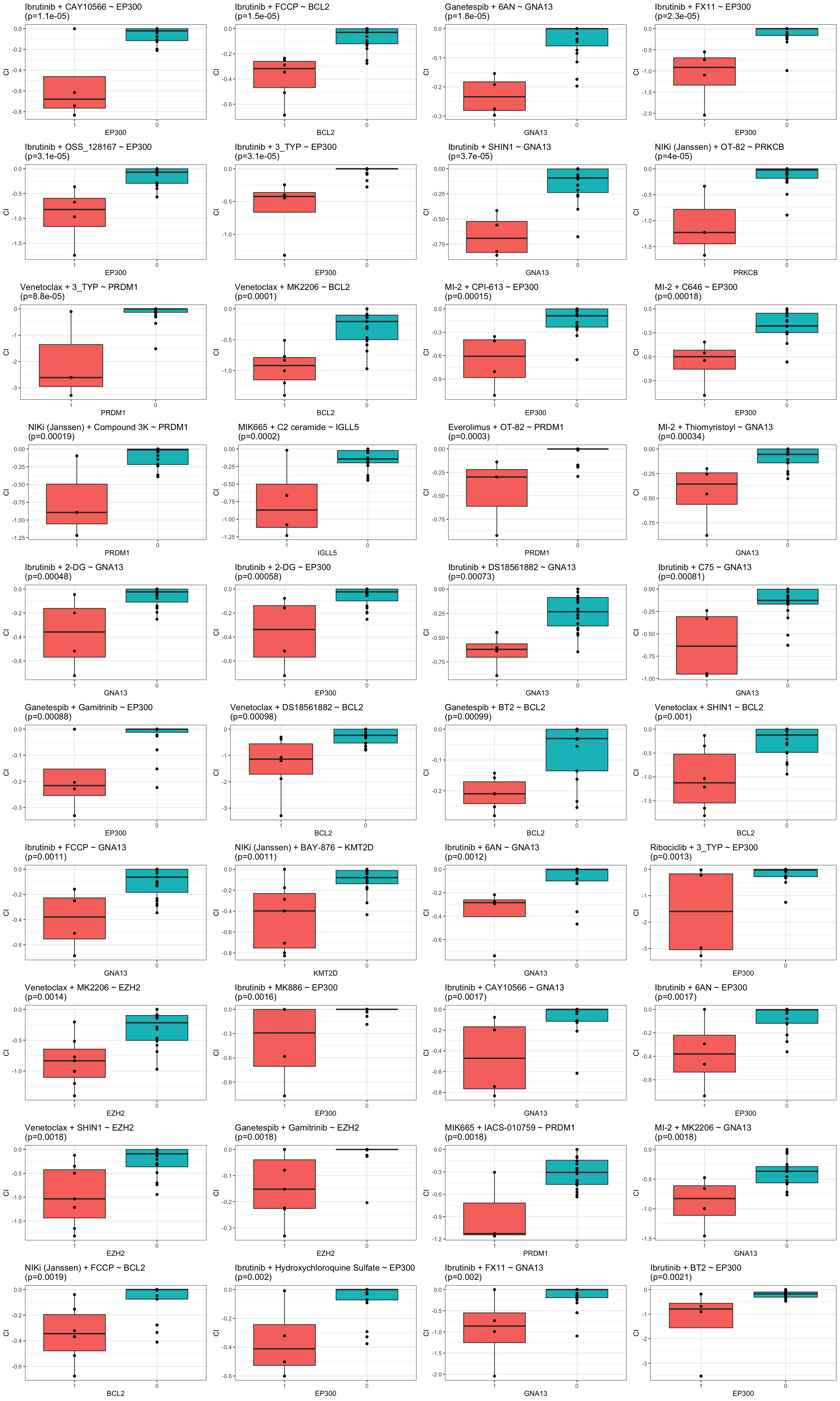

Correlate combination effect with clinical drug responses

Test per concentration

resTab.conc <- synTab %>% filter(!is.na(viabA), !is.na(CI)) %>%
  group_by(Drug_A, Drug_A.Conc, Drug_A.ConcStep,
                        Drug_B, Drug_B.ConcStep) %>% nest() %>%
  mutate(m = map(data, ~cor.test(~CI+viabA,.,method = "spearman"))) %>%
  mutate(res = map(m, broom::tidy)) %>%
  unnest(res) %>% ungroup() %>%
  arrange(p.value) %>%
  group_by(Drug_A) %>%
  mutate(p.adj = p.adjust(p.value, method = "BH"))

P-value histogram per clinical drug

ggplot(resTab.conc, aes(x=p.value)) +
  geom_histogram(aes(fill = Drug_A), alpha=0.5, color = "black") +
  facet_wrap(~Drug_A) +
  theme_bw() +
  theme(legend.position = "none")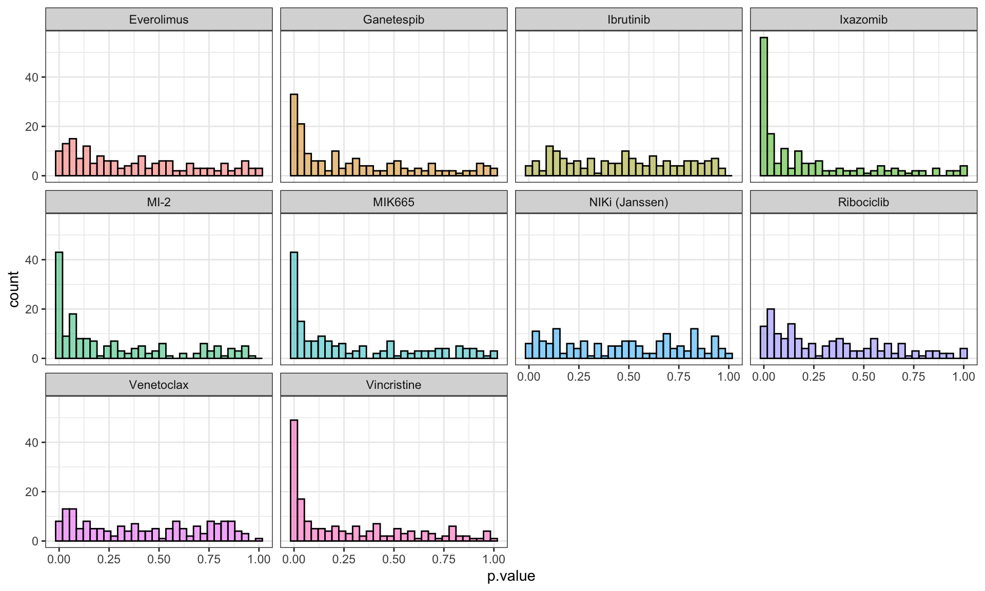

Correlation coefficient distribution

ggplot(resTab.conc, aes(x=estimate, fill = Drug_A)) +
  geom_density(alpha =0.5) +
  facet_wrap(~Drug_A) +
  geom_vline(xintercept = 0, linetype = "dashed", color ="red") +
  theme(legend.position = "none") +
  xlab("Correlation coefficient")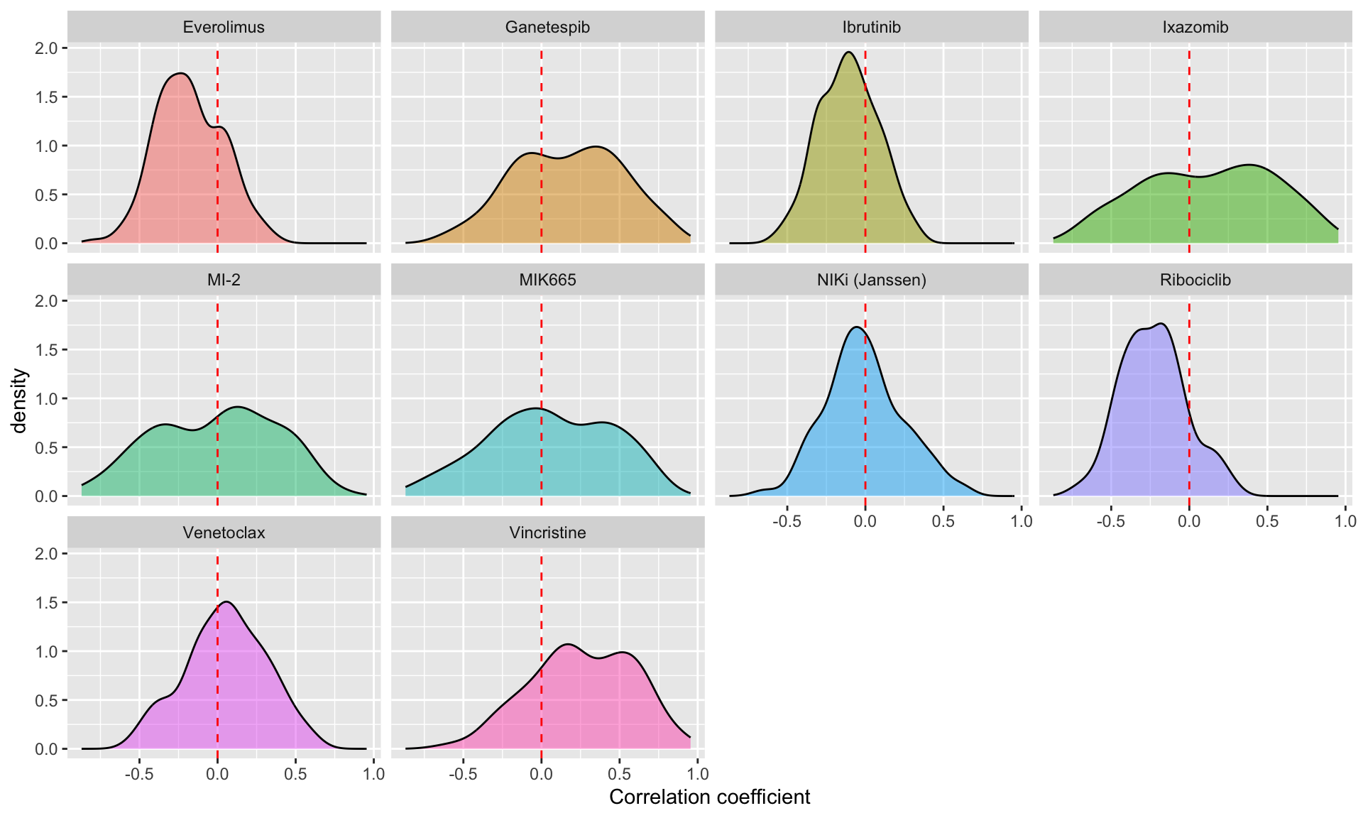

P-value heatmap

plotTab <- select(resTab.conc, Drug_A, Drug_B, Drug_A.ConcStep, estimate, p.value, p.adj) %>%
  mutate(Psign = sign(estimate)*(-log10(p.value))) %>%
  mutate(ifSig = ifelse(p.adj <= 0.10, "*",""))

ggplot(plotTab, aes(x=Drug_A.ConcStep, y=Drug_B, fill = Psign)) +
  geom_tile() +
  geom_text(aes(label = ifSig), vjust =0.5) +
  scale_fill_gradient2() +
  facet_wrap(~Drug_A, nrow=1)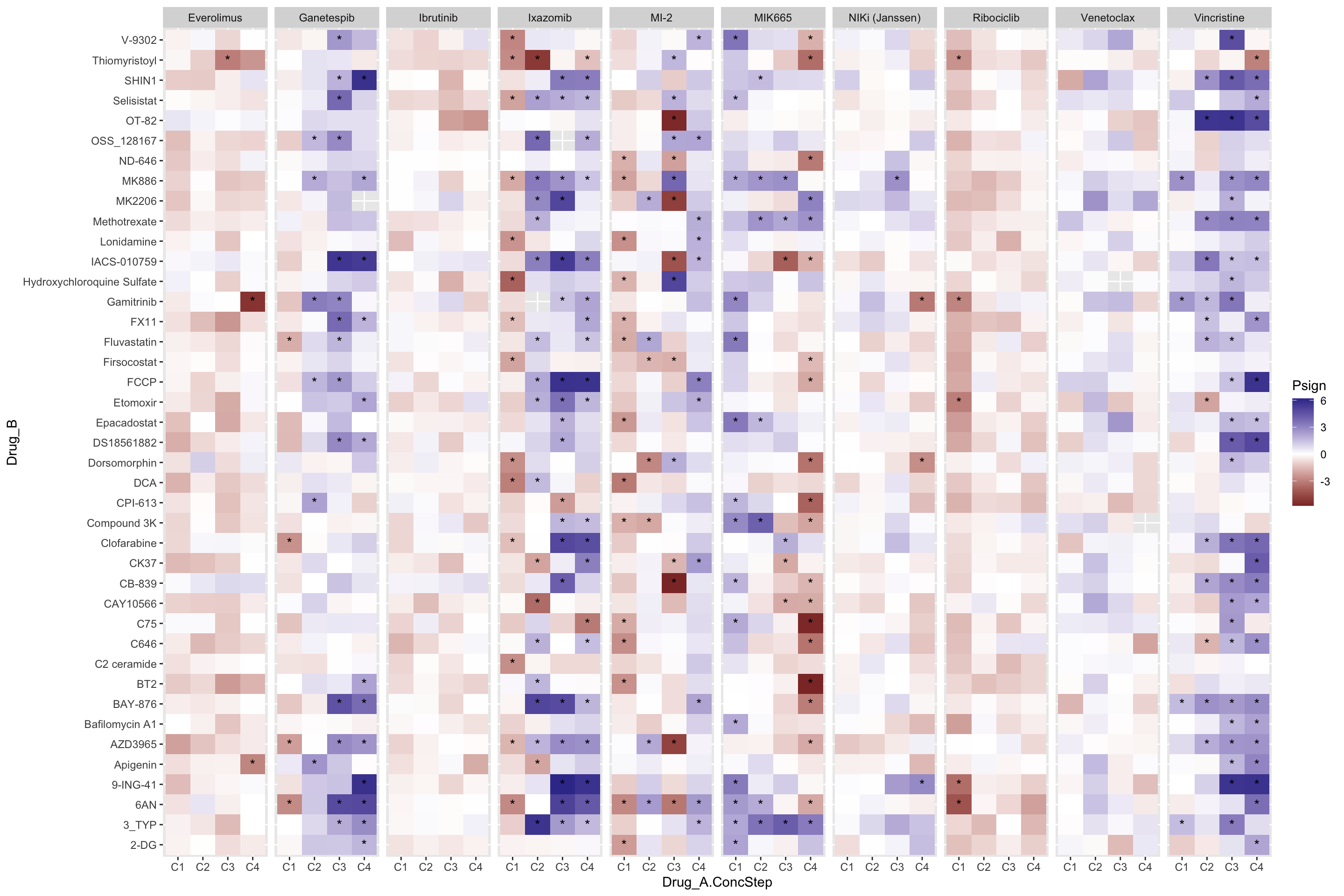

Scatter plot of significant associations

Top 20 negative associations: higher resistance correlated with lower CI (more synergistic)

plotDrug <- filter(resTab.conc, estimate <0)
pList <- lapply(seq(20), function(i) {
  rec <- plotDrug[i,]
  plotTab <- filter(synTab, Drug_A == rec$Drug_A, Drug_B == rec$Drug_B,
                    Drug_A.ConcStep == rec$Drug_A.ConcStep)
  ggplot(plotTab, aes(x=viabA, y=CI)) +
    geom_point() + geom_smooth(method="lm") +
    ggtitle(sprintf("%s ~ %s\n(concStep: %s)", rec$Drug_A, rec$Drug_B, rec$Drug_A.ConcStep)) +
    xlab(rec$Drug_A) +
    theme_bw()
})
cowplot::plot_grid(plotlist = pList, ncol=4)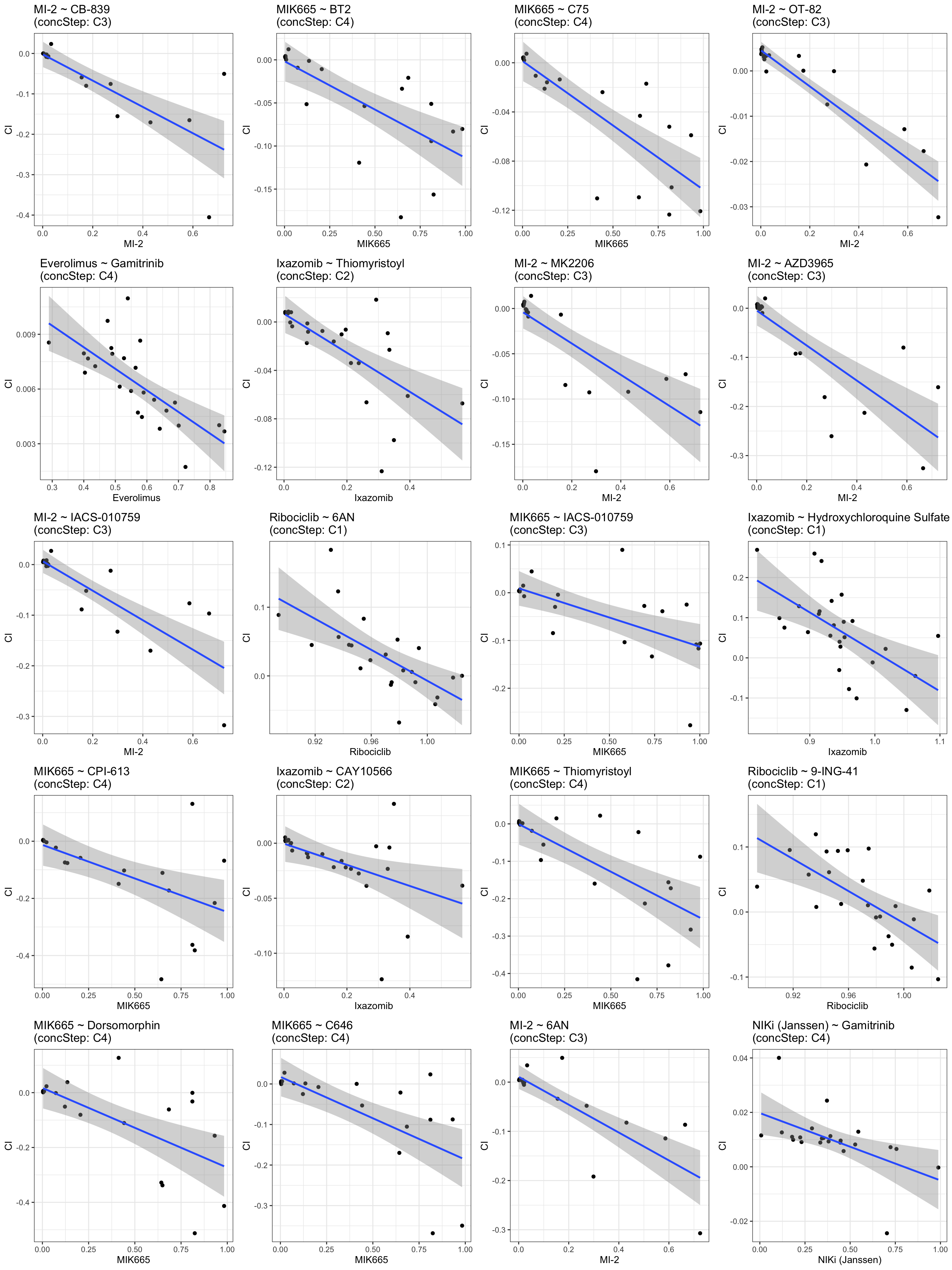

Top 9 positive associations: higher resistance correlated with higher CI (more antagonistic)

plotDrug <- filter(resTab.conc, estimate >0)
pList <- lapply(seq(20), function(i) {
  rec <- plotDrug[i,]
  plotTab <- filter(synTab, Drug_A == rec$Drug_A, Drug_B == rec$Drug_B,
                    Drug_A.ConcStep == rec$Drug_A.ConcStep)
  ggplot(plotTab, aes(x=viabA, y=CI)) +
    geom_point() + geom_smooth(method="lm") +
    ggtitle(sprintf("%s ~ %s\n(concStep: %s)", rec$Drug_A, rec$Drug_B, rec$Drug_A.ConcStep)) +
    xlab(rec$Drug_A) +
    theme_bw()
})
cowplot::plot_grid(plotlist = pList, ncol=4)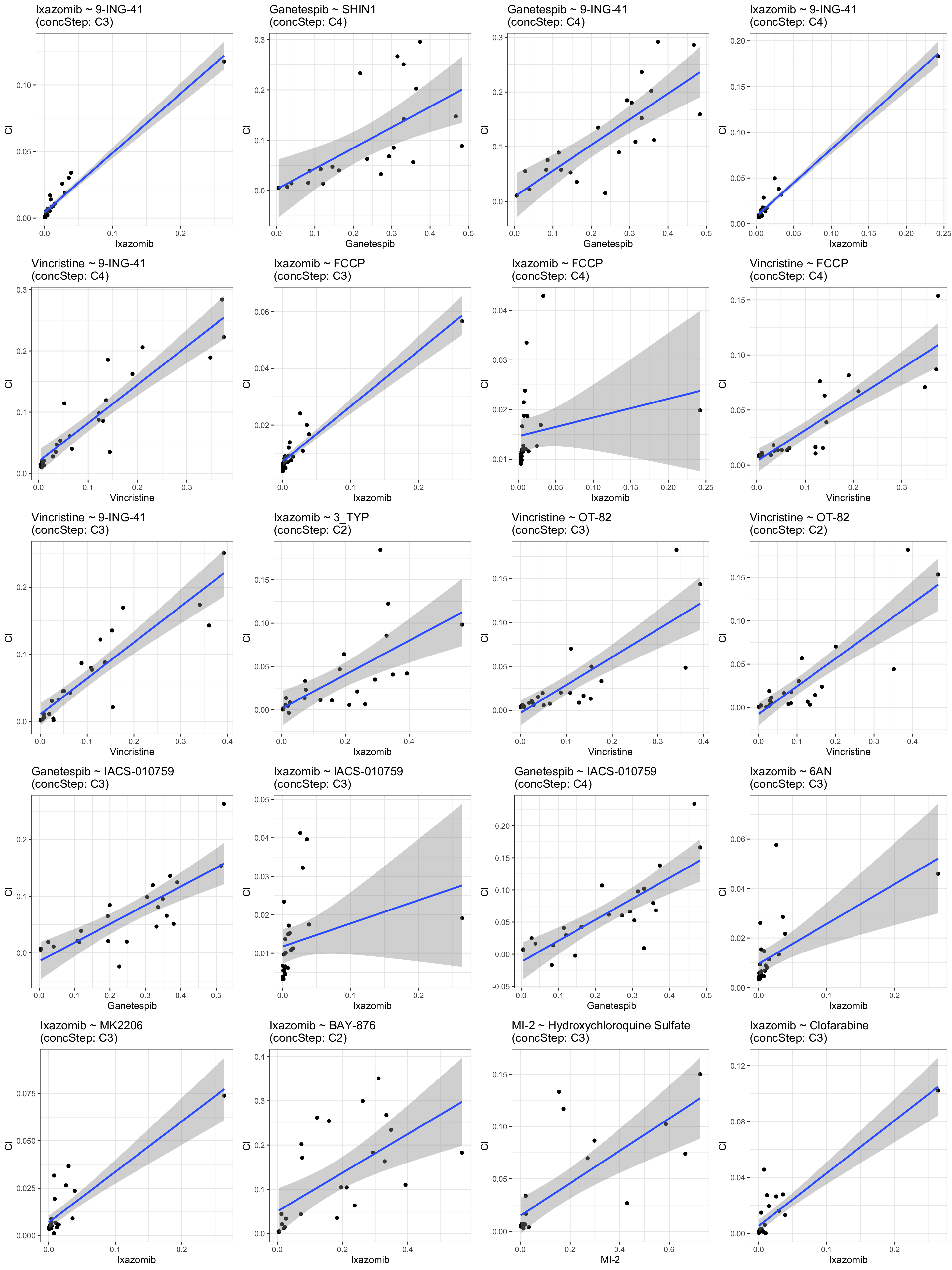

At summarised level

Use AUC for the clinical drug responses and summarised CI for combinations

Calculate AUC for clinical drugs

viabA <- drugATab %>% group_by(Name, Drug_A) %>%
  summarise(auc = calcAUC(viabA, Drug_A.Conc))

Correlate AUC with summarised CI

testTab <- viabA %>% left_join(ciTabSum, by = c("Drug_A","Name")) %>%
  pivot_longer(c(syn, anta), names_to = "type", values_to = "score") %>%
  filter(!is.na(auc), !is.na(score))

resTab.sum <- group_by(testTab, Drug_A, Drug_B, type) %>%
  nest() %>%
  mutate(m = map(data, ~cor.test(~auc+score,., method = "spearman"))) %>%
  mutate(res = map(m, broom::tidy)) %>%
  unnest(res) %>%
  group_by(type, Drug_A) %>%
  mutate(p.adj = p.adjust(p.value, method = "BH")) %>%
  ungroup() %>% arrange(p.value)

P-value histogram per clinical drug

ggplot(resTab.sum, aes(x=p.value)) +
  geom_histogram(aes(fill = Drug_A), alpha=0.5, color = "black") +
  facet_wrap(~Drug_A+type, scale = "free_y", ncol=4) +
  theme_bw() +
  theme(legend.position = "none")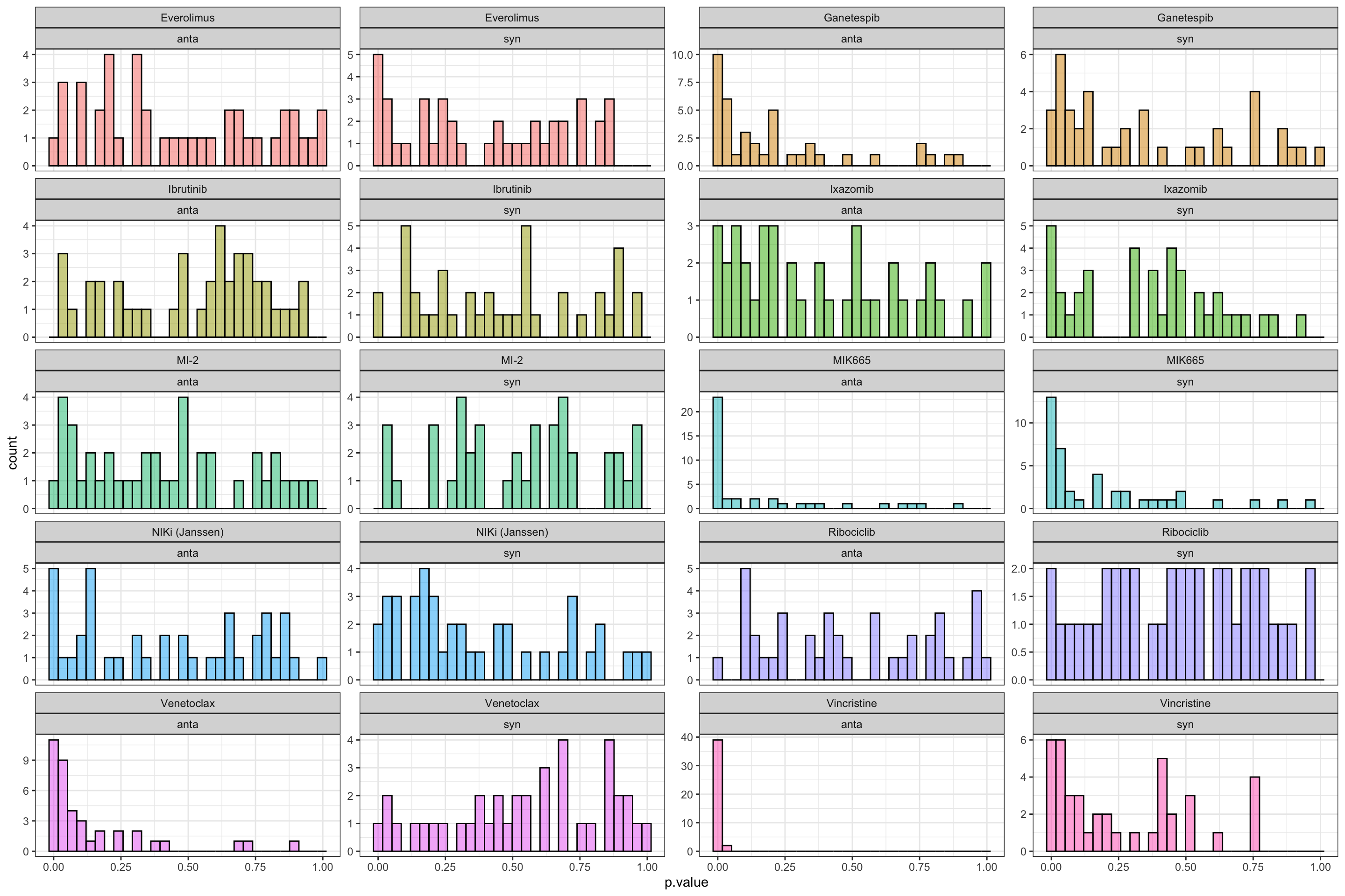

Correlation coefficient distribution

ggplot(resTab.sum, aes(x=estimate, fill = Drug_A)) +
  geom_density(alpha =0.5) +
  facet_wrap(~Drug_A+type, ncol=4) +
  geom_vline(xintercept = 0, linetype = "dashed", color ="red") +
  theme(legend.position = "none") +
  xlab("Correlation coefficient")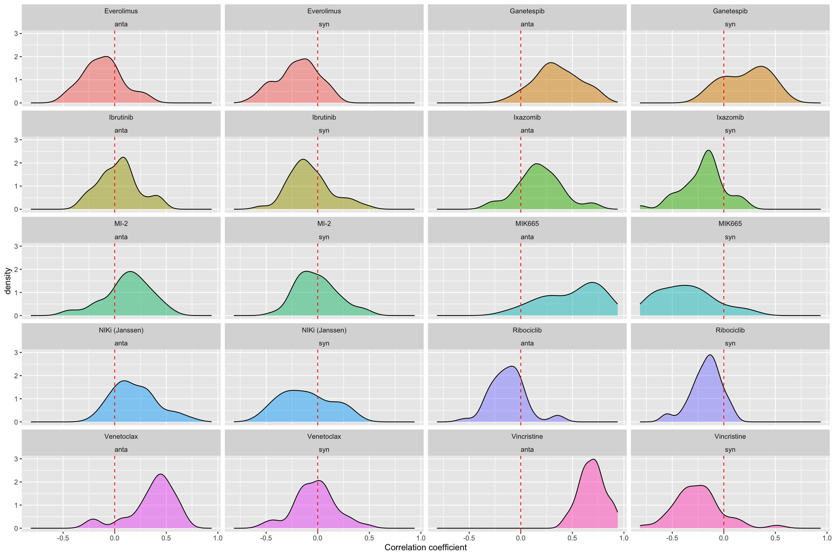

P-value heatmap

plotTab <- select(resTab.sum, Drug_A, Drug_B, estimate, p.value, p.adj,type) %>%
  mutate(Psign = sign(estimate)*(-log10(p.value))) %>%
  mutate(ifSig = ifelse(p.adj <= 0.10, "*",""))

ggplot(plotTab, aes(x=Drug_A, y=Drug_B, fill = Psign)) +
  geom_tile() +
  geom_text(aes(label = ifSig), vjust =0.5) +
  scale_fill_gradient2() +
  facet_wrap(~type, nrow=1) +
  theme(axis.text.x = element_text(angle = 90, hjust = 1, vjust = 0.5))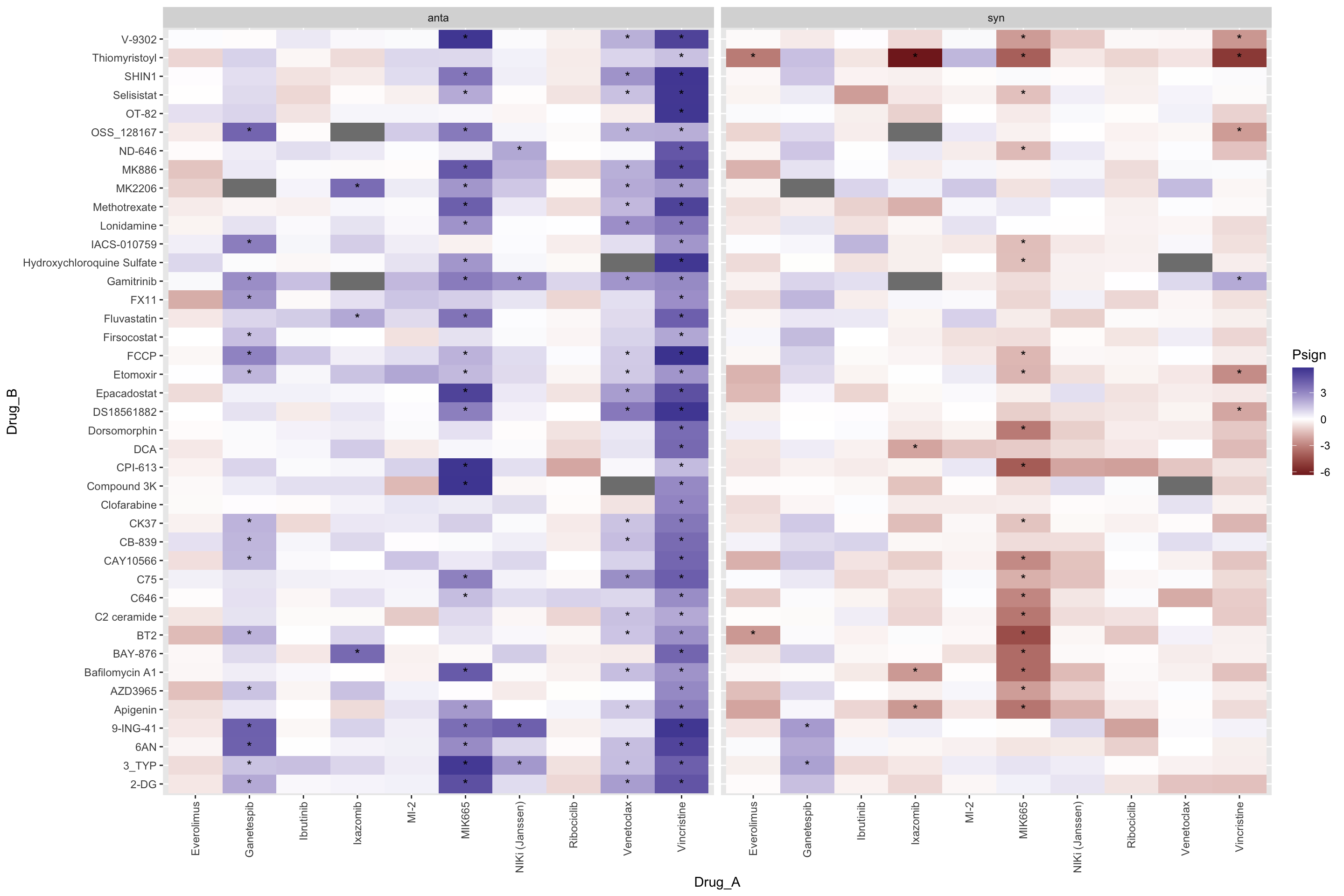

Scatter plot of significant associations

Top 20 negative associations with synergy: higher resistance correlated with higher synergy

plotDrug <- filter(resTab.sum, estimate <0, type =="syn")
pList <- lapply(seq(20), function(i) {
  rec <- plotDrug[i,]
  plotTab <- filter(testTab, Drug_A == rec$Drug_A, Drug_B == rec$Drug_B,
                    type == rec$type)
  ggplot(plotTab, aes(x=auc, y=score)) +
    geom_point() + geom_smooth(method="lm") +
    ggtitle(sprintf("%s ~ %s (synergy)", rec$Drug_A, rec$Drug_B)) +
    xlab(rec$Drug_A) +
    theme_bw()
})
cowplot::plot_grid(plotlist = pList, ncol=4)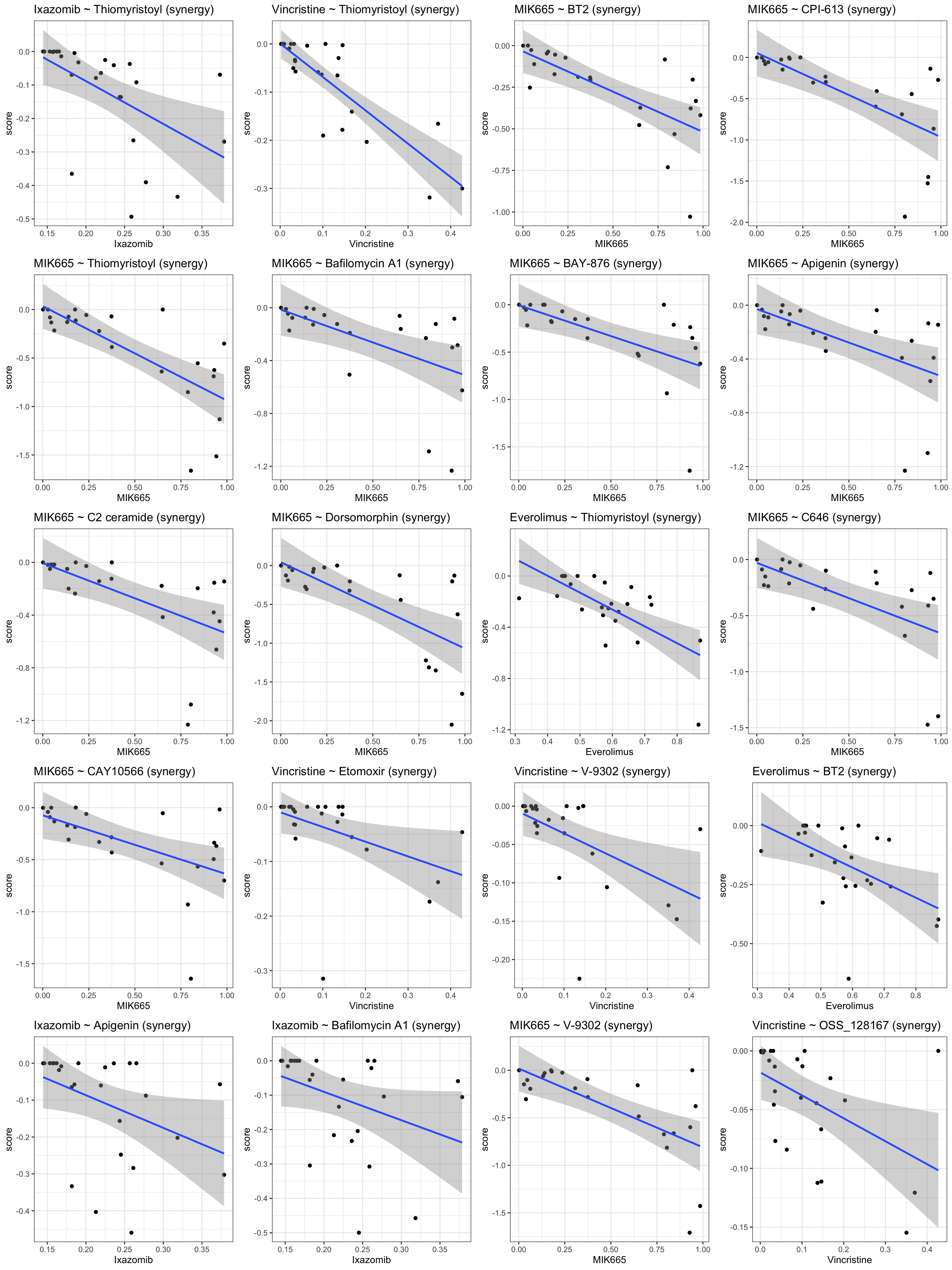

Top 20 positive associations with antagonistic: higher resistance correlated with more antagonistic effect

plotDrug <- filter(resTab.sum, estimate >0, type =="anta")
pList <- lapply(seq(20), function(i) {
  rec <- plotDrug[i,]
  plotTab <- filter(testTab, Drug_A == rec$Drug_A, Drug_B == rec$Drug_B,
                    type == rec$type)
  ggplot(plotTab, aes(x=auc, y=score)) +
    geom_point() + geom_smooth(method="lm") +
    ggtitle(sprintf("%s ~ %s (antagonistic)", rec$Drug_A, rec$Drug_B)) +
    xlab(rec$Drug_A) +
    theme_bw()
})
cowplot::plot_grid(plotlist = pList, ncol=4)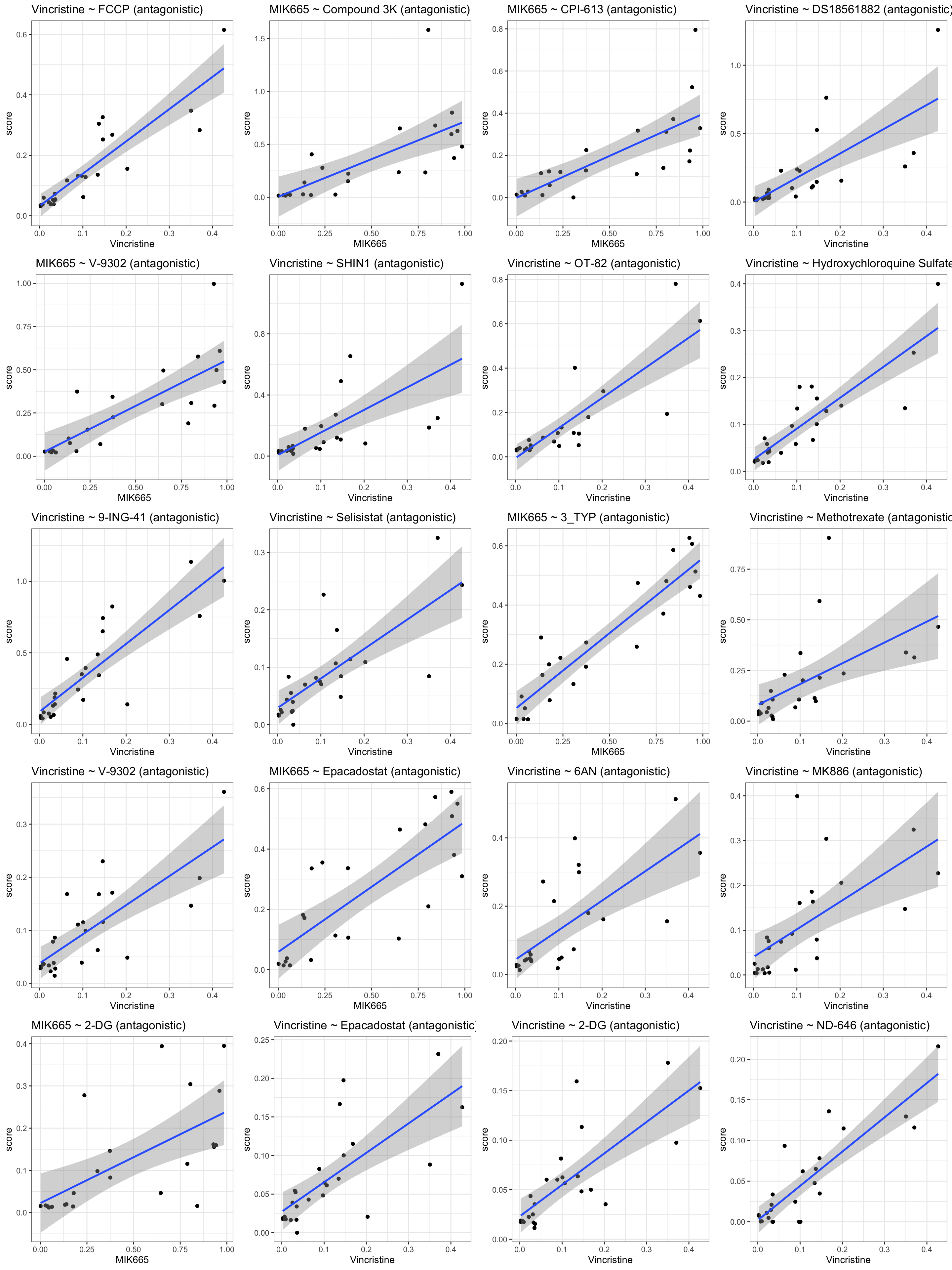

Define non-responder cell lines and test for synergy

Define non-responders to clinical drugs using the mirror method proposed by Wolfgang

Plot response distribution for each clinical drug

ggplot(viabA, aes(x=auc)) + geom_histogram() + facet_wrap(~Drug_A)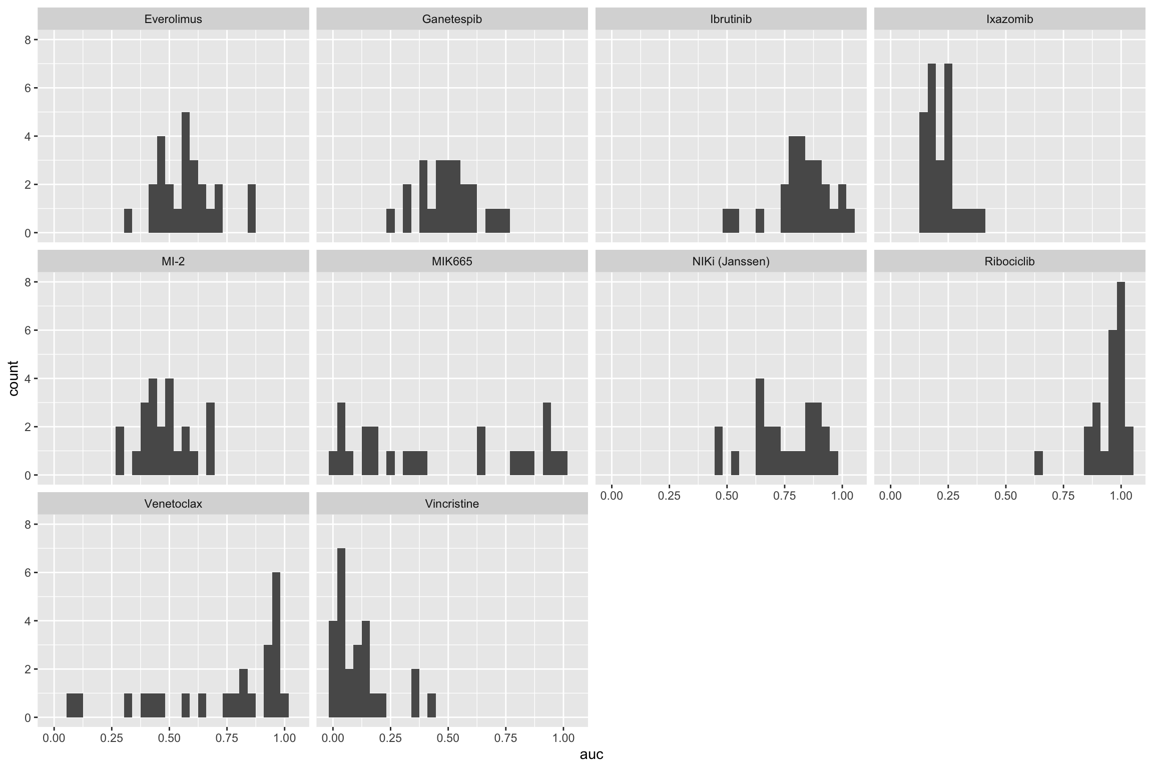

The mirro method may not work for this dataset. Perhaps it’s better to just define the response group manually?

Comapre BayeSynergy score with Bliss synergy score

Load BayeSynergy score calcualted by Antonia

load("../output/fit_BayeSynergy_AA.rdata")
comTabCI <- fit$screenSummary %>% 
  select(`Experiment ID`,  `Drug A`, `Drug B`, `Synergy Score`, `Antagonism Score`) %>%
  dplyr::rename(Name = `Experiment ID`, Drug_A = `Drug A`, Drug_B = `Drug B`, syn = `Synergy Score`, anta = `Antagonism Score`) %>%
  mutate(model = "BayeSynergy") %>%
  bind_rows(mutate(ciTabSum, model = "Bliss")) %>%
  pivot_longer(c(syn,anta), names_to = "type", values_to = "score") %>%
  pivot_wider(names_from = model, values_from = score)

Overall comparison

ggplot(comTabCI, aes(x=Bliss, y=BayeSynergy)) +
  geom_point(aes(color = type)) +
  theme_bw()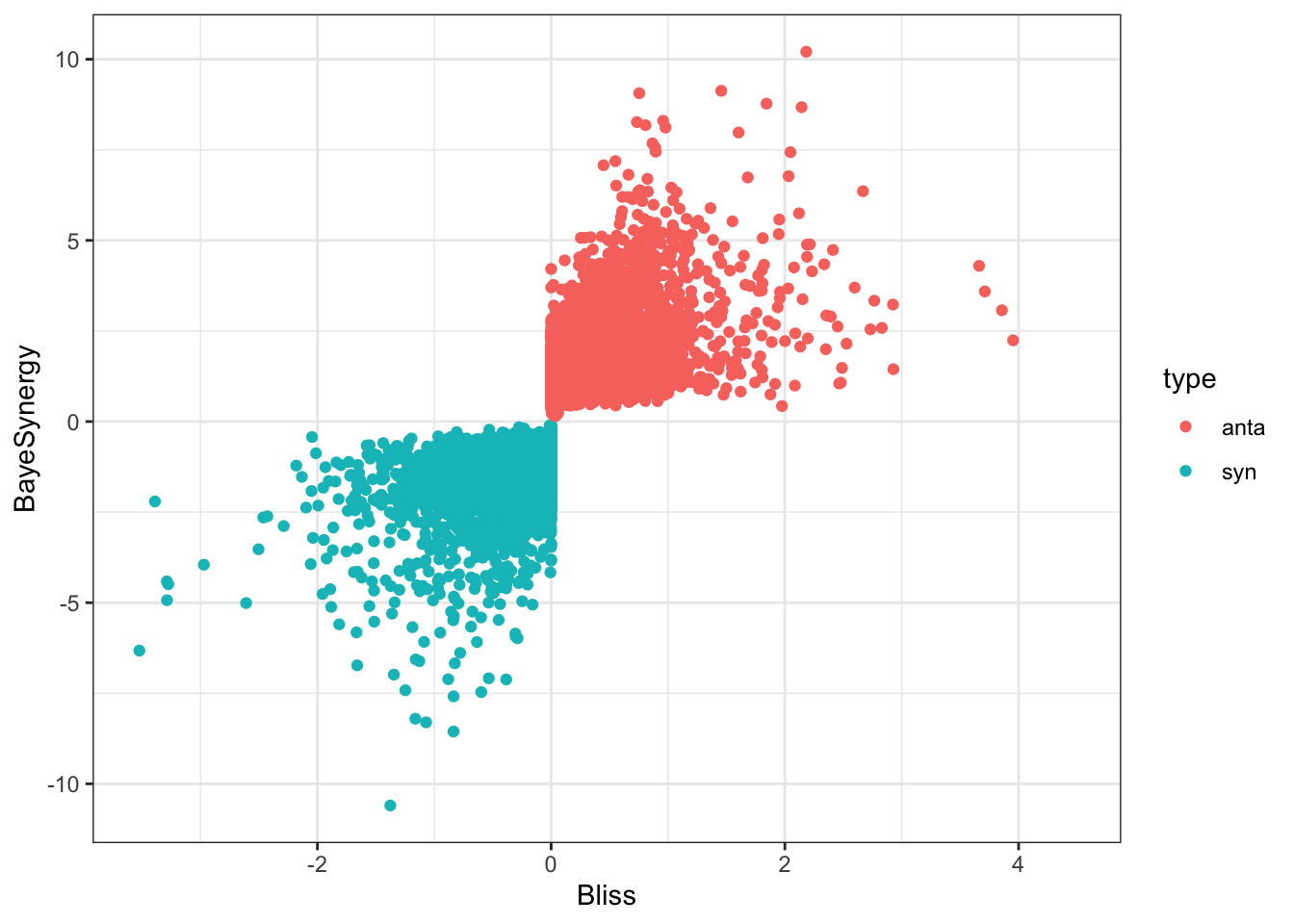

Overall the synergy and antagonistic scores from Bliss models and Bayesynergy are comparable.

Visualize per cellline + clinical drug

pList <- lapply(unique(comTabCI$Drug_A), function(drugA) {
  
  plotTab <- filter(comTabCI, Drug_A == drugA) %>% filter(!is.na(BayeSynergy), !is.na(Bliss))
  
  #label the top 5 CIs by either BayeSynergy or Bliss
  selectTopN <- function(tab, n=3) {
     topBayes <- arrange(tab, desc(abs(BayeSynergy)))$Drug_B[seq(n)]
     topBliss <- arrange(tab, desc(abs(Bliss)))$Drug_B[seq(n)]
     return(tibble(drugName = unique(c(topBayes, topBliss))))
  }
  topDrug <- group_by(plotTab, Name, Drug_A, type) %>% nest() %>%
    mutate(res = map(data, selectTopN)) %>%
    unnest(res) %>%
    select(-data) %>%
    mutate(Drug_B = drugName)
  
  plotTab <- left_join(plotTab, topDrug, by = c("Name","Drug_A","type","Drug_B"))
  
  ggplot(plotTab, aes(x=Bliss, y=BayeSynergy)) +
    geom_point(aes(color = type)) +
    facet_wrap(~Name, ncol=5) +
    ggrepel::geom_text_repel(aes(label = drugName), max.overlaps = Inf) +
    theme_bw() +
    geom_hline(yintercept = 0, linetype = "dashed", color = "grey50") +
    geom_vline(xintercept = 0, linetype = "dashed", color = "grey50") +
    ggtitle(drugA) +
    theme(plot.title = element_text(hjust = 0.5,size = 20, face="bold"))
    
})
jyluMisc::makepdf(pList,"../docs/comapre_Bliss_BayeSynergy.pdf",ncol=1, nrow=1, width = 15, height = 15)

comapre_Bliss_BayeSynergy.pdf
The top 5 synergy and antagonism from either Bliss or Bayesynergy are labeled.

Multi-variate regression to identfy associations between genomics and synergy

Bliss synergy

Prepare genomic table

mutMat <- mutTab %>% pivot_wider(names_from = Gene, values_from = status)

Selected drug pairs for visualization

selectedPair <- tibble(Drug_A = c("MI-2","MI-2","MIK665","MIK665","Ixazomib","Ixazomib"),
                   Drug_B = c("AZD3965","IACS-010759","AZD3965","IACS-010759","BT2","C2 ceramide"))

Multi-variate linear regression for each combination

drugPair <- ungroup(ciTabSum) %>% distinct(Drug_A, Drug_B) #test for all drug pairs

allRes <- BiocParallel::bplapply(seq(nrow(drugPair)), function(i) {
  rec <- drugPair[i,]
  synVal <- filter(ciTabSum, Drug_A == rec$Drug_A, Drug_B==rec$Drug_B) %>%
    ungroup() %>%
    select(Name, syn)
  testTab <- left_join(mutMat, synVal, by = "Name") %>%
    column_to_rownames("Name")
  m <- summary(lm(syn ~ ., testTab))
  R2 <- m$r.squared
  coefTab <- m$coefficients[-1,c(1,4)] %>% data.frame() %>%
    rownames_to_column("Gene") %>%
    as_tibble() %>%
    dplyr::rename(p = "Pr...t..")
  #colnames(coefTab) <- c("coef","p")
  tibble(Drug_A = rec$Drug_A, Drug_B = rec$Drug_B, R2 = R2, coefTab = list(coefTab)) %>%
    mutate(R2 = replace_na(R2,0))
}) %>%
  bind_rows() %>% arrange(desc(R2)) %>% mutate(combination = paste0(Drug_A,"_", Drug_B))

seleRes <- allRes %>% filter(combination %in% paste0(selectedPair$Drug_A,"_",selectedPair$Drug_B))

Variance explained (R2) for each selected synergy by genomics

plotTab <- seleRes %>%
  mutate(combination = factor(combination, levels = combination))
ggplot(plotTab, aes(x=combination, y=R2)) +
  geom_bar(aes(fill = combination), stat = "identity") + 
  coord_flip() +
  theme(legend.position = "none")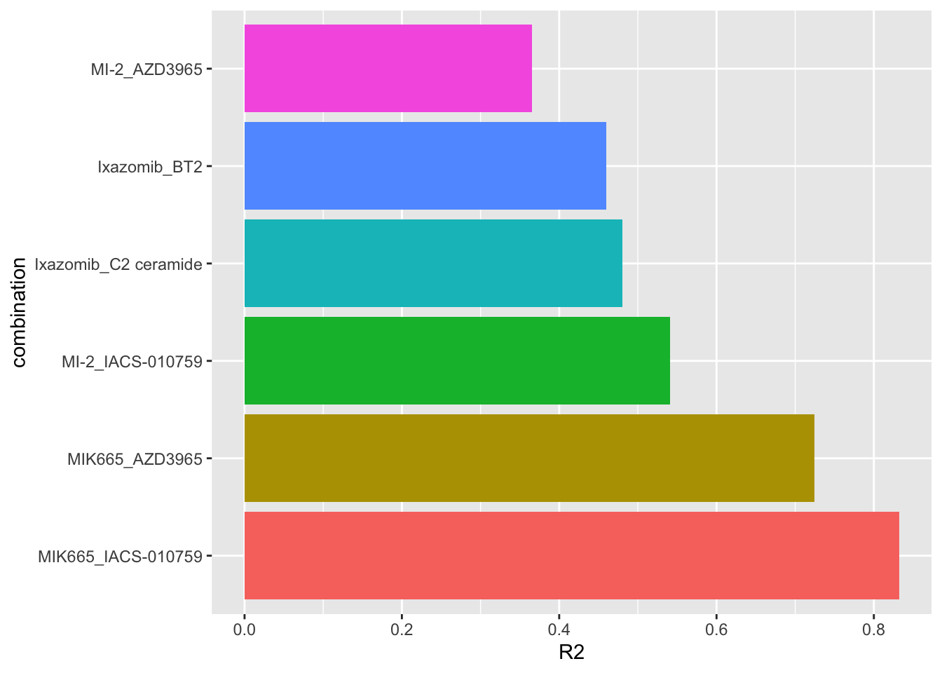

Genes that can explain synergy in multi-variate models (for selected drug pairs)

plotTab <- unnest(seleRes, coefTab) %>%
  mutate(ifSig = ifelse(p <= 0.05, ifelse(p<=0.01,"**","*"),"")) %>%
  mutate(combination = sprintf("%s_%s (R2=%1.1f)",Drug_A, Drug_B, R2))

ggplot(plotTab, aes(x=Gene, y=combination, fill = Estimate)) +
  geom_tile() +
  geom_text(aes(label = ifSig)) +
  scale_fill_gradient2(low = "blue", high = "red", mid="white", midpoint = 0, name ="coefficient")+
  ggtitle("Selected drug pairs") +
  theme(axis.text.x = element_text(angle = 90, hjust = 1, vjust = 0.5),
        plot.title = element_text(face = "bold", hjust = 0.5))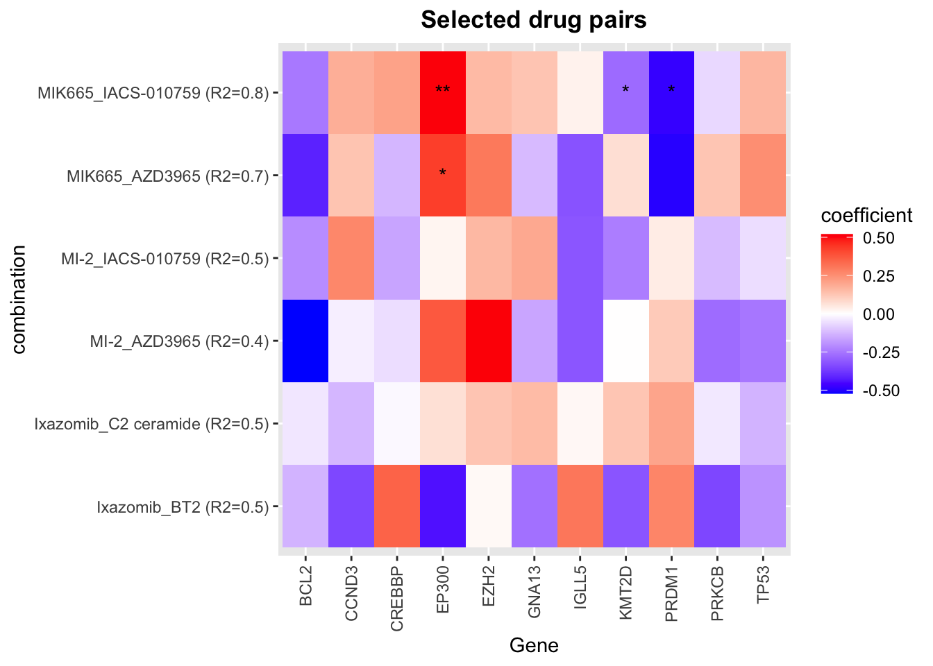

Color of the heatmap indicates the coefficients of the genomic features in the multi-variate regression model to explain the CI scores. Since higher CI score is associated with higher synergy, negative coefficient (blue tiles) indicates the mutations associate with higher synergy and positive coefficient (red tiles) indicates mutations associate with lower synergy.
R2 values indicate how much variance in the synergistic scores can be explained by the genomics
* indicates the significance of the genomic features in the multi-variate models. One star is p < 0.05 and two starts indicate p<0.01.

Genes that can explain synergy in multi-variate models (for all drug pairs)

pList <- lapply(unique(allRes$Drug_A), function(name) {
  plotTab <- filter(allRes, Drug_A == name) %>%
    unnest(coefTab) %>%
    mutate(ifSig = ifelse(p <= 0.05, ifelse(p<=0.01,"**","*"),"")) %>% 
    mutate(combination = sprintf("%s_%s (R2=%1.1f)",Drug_A, Drug_B, R2)) %>%
    arrange(R2) %>% mutate(combination = factor(combination, levels = unique(combination)))

  ggplot(plotTab, aes(x=Gene, y=combination, fill = Estimate)) +
    geom_tile() +
    geom_text(aes(label = ifSig)) +
    scale_fill_gradient2(low = "blue", high = "red", mid="white", midpoint = 0, name ="coefficient")+
    ggtitle(name) +
    theme(axis.text.x = element_text(angle = 90, hjust = 1, vjust = 0.5),
          plot.title = element_text(face = "bold", hjust = 0.5)) 
})
jyluMisc::makepdf(pList, "../docs/multiVariate_GeneAssociation_Bliss.pdf", 
                  ncol = 1, nrow = 1,
                  height = 10, width = 10)

PDF plot

Bayes synergy

load("../output/fit_BayeSynergy_AA.rdata")
bayesTabSum <- fit$screenSummary %>% 
  select(`Experiment ID`,  `Drug A`, `Drug B`, `Synergy Score`, `Antagonism Score`) %>%
  dplyr::rename(Name = `Experiment ID`, Drug_A = `Drug A`, Drug_B = `Drug B`, syn = `Synergy Score`, anta = `Antagonism Score`)

Multi-variate linear regression for each combination

drugPair <- ungroup(bayesTabSum) %>% distinct(Drug_A, Drug_B) #test for all drug pairs

allRes <- BiocParallel::bplapply(seq(nrow(drugPair)), function(i) {
  rec <- drugPair[i,]
  synVal <- filter(bayesTabSum, Drug_A == rec$Drug_A, Drug_B==rec$Drug_B) %>%
    ungroup() %>%
    select(Name, syn)
  testTab <- left_join(mutMat, synVal, by = "Name") %>%
    column_to_rownames("Name")
  m <- summary(lm(syn ~ ., testTab))
  R2 <- m$r.squared
  coefTab <- m$coefficients[-1,c(1,4)] %>% data.frame() %>%
    rownames_to_column("Gene") %>%
    as_tibble() %>%
    dplyr::rename(p = "Pr...t..")
  #colnames(coefTab) <- c("coef","p")
  tibble(Drug_A = rec$Drug_A, Drug_B = rec$Drug_B, R2 = R2, coefTab = list(coefTab)) %>%
    mutate(R2 = replace_na(R2,0))
}) %>%
  bind_rows() %>% arrange(desc(R2)) %>% mutate(combination = paste0(Drug_A,"_", Drug_B))

seleRes <- allRes %>% filter(combination %in% paste0(selectedPair$Drug_A,"_",selectedPair$Drug_B))

Variance explained (R2) for each selected synergy by genomics

plotTab <- seleRes %>%
  mutate(combination = factor(combination, levels = combination))
ggplot(plotTab, aes(x=combination, y=R2)) +
  geom_bar(aes(fill = combination), stat = "identity") + 
  coord_flip() +
  theme(legend.position = "none")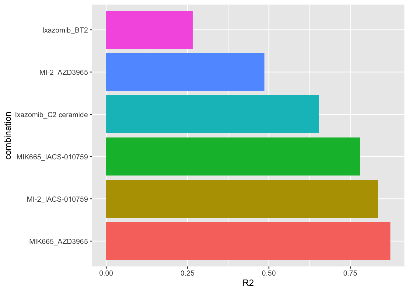

Genes that can explain synergy in multi-variate models (for selected drug pairs)

plotTab <- unnest(seleRes, coefTab) %>%
  mutate(ifSig = ifelse(p <= 0.05, ifelse(p<=0.01,"**","*"),"")) %>%
  mutate(combination = sprintf("%s_%s (R2=%1.1f)",Drug_A, Drug_B, R2))

ggplot(plotTab, aes(x=Gene, y=combination, fill = Estimate)) +
  geom_tile() +
  geom_text(aes(label = ifSig)) +
  scale_fill_gradient2(low = "blue", high = "red", mid="white", midpoint = 0, name ="coefficient")+
  ggtitle("Selected drug pairs") +
  theme(axis.text.x = element_text(angle = 90, hjust = 1, vjust = 0.5),
        plot.title = element_text(face = "bold", hjust = 0.5))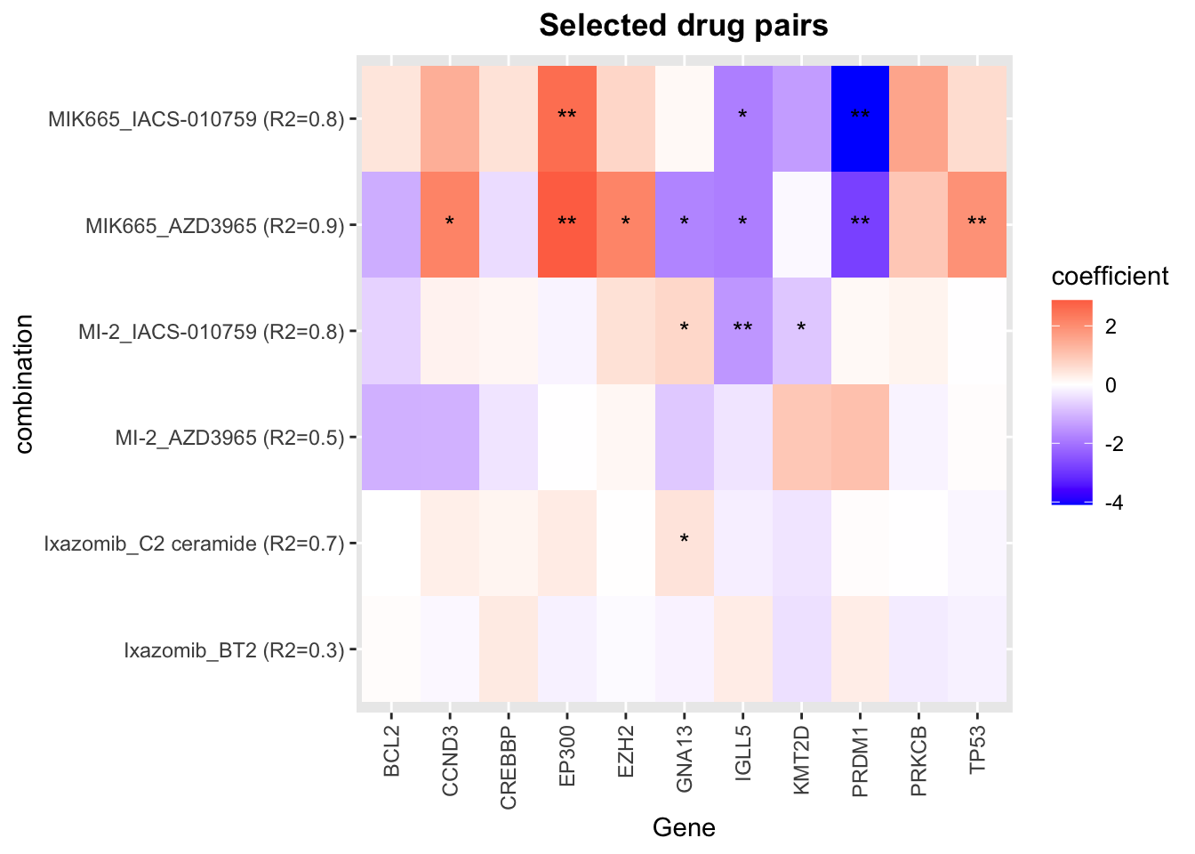

Color of the heatmap indicates the coefficients of the genomic features in the multi-variate regression model to explain the CI scores. Since higher CI score is associated with higher synergy, negative coefficient (blue tiles) indicates the mutations associate with higher synergy and positive coefficient (red tiles) indicates mutations associate with lower synergy.
R2 values indicate how much variance in the synergistic scores can be explained by the genomics
* indicates the significance of the genomic features in the multi-variate models. One star is p < 0.05 and two starts indicate p<0.01.

Genes that can explain synergy in multi-variate models (for all drug pairs)

pList <- lapply(unique(allRes$Drug_A), function(name) {
  plotTab <- filter(allRes, Drug_A == name) %>%
    unnest(coefTab) %>%
    mutate(ifSig = ifelse(p <= 0.05, ifelse(p<=0.01,"**","*"),"")) %>% 
    mutate(combination = sprintf("%s_%s (R2=%1.1f)",Drug_A, Drug_B, R2)) %>%
    arrange(R2) %>% mutate(combination = factor(combination, levels = unique(combination)))

  ggplot(plotTab, aes(x=Gene, y=combination, fill = Estimate)) +
    geom_tile() +
    geom_text(aes(label = ifSig)) +
    scale_fill_gradient2(low = "blue", high = "red", mid="white", midpoint = 0, name ="coefficient")+
    ggtitle(name) +
    theme(axis.text.x = element_text(angle = 90, hjust = 1, vjust = 0.5),
          plot.title = element_text(face = "bold", hjust = 0.5)) 
})
jyluMisc::makepdf(pList, "../docs/multiVariate_GeneAssociation_Bayesynergy.pdf", 
                  ncol = 1, nrow = 1,
                  height = 10, width = 10)

PDF plot

Explain synergy score by transcriptomics

Processing transcriptomic data

Number of genes and cell lines

load("../data/DepMap_GEXwide.RData")
exprMat <- t(DepMap_GEXwide)
exprMat <- exprMat[,colnames(exprMat) %in% unique(ciTabSum$Name)]

# Remove low count genes
exprMat <- exprMat[matrixStats::rowMedians(exprMat) >0,]

vstObj <- vsn::vsnMatrix(exprMat)
exprMat <- vsn::predict(vstObj, exprMat)

dim(exprMat)

[1] 15631    12

Using Bliss synergy

Prepare list of selected synergy scores

synList <- ciTabSum %>%
  mutate(combination = paste0(Drug_A, "_", Drug_B)) %>% 
  filter(combination %in% paste0(selectedPair$Drug_A,"_",selectedPair$Drug_B)) %>%
  mutate(score = syn)

Perform association tests

allRes <- predictSynergy(synList, exprMat)

P-value histogram

ggplot(allRes, aes(x=P.Value)) +
  geom_histogram() +
  facet_wrap(~combination)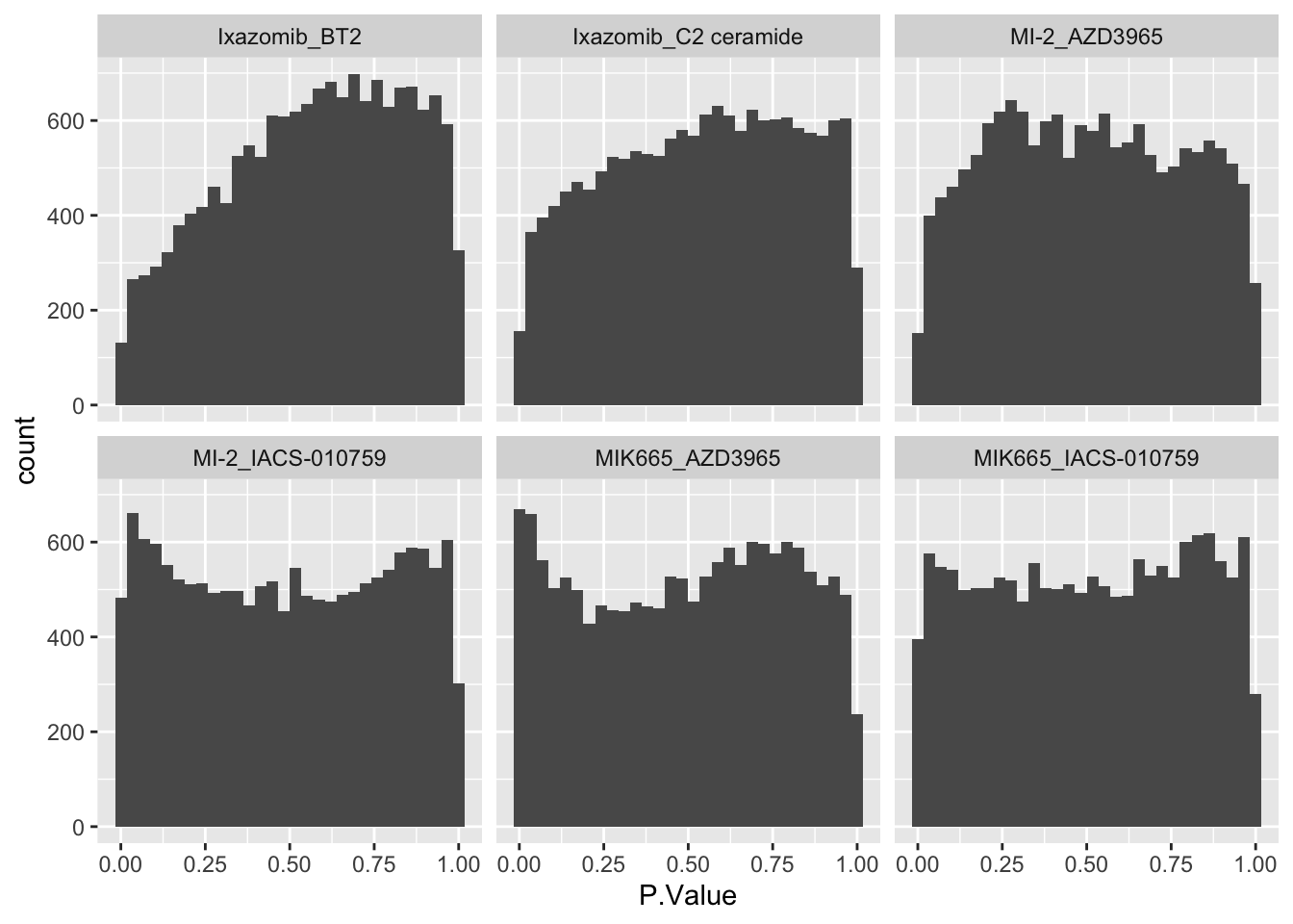

Number of significant associations

Use 10% FDR (adj.P.Val < 0.1)

sumTab <- group_by(allRes, combination) %>%
  summarise(num = sum(adj.P.Val <= 0.10))
sumTab

# A tibble: 6 × 2
  combination            num
  <chr>                <int>
1 Ixazomib_BT2             0
2 Ixazomib_C2 ceramide     0
3 MI-2_AZD3965             0
4 MI-2_IACS-010759         0
5 MIK665_AZD3965         179
6 MIK665_IACS-010759       0

Use raw P.Value < 0.01 (without multiple hypothesis adjustment)

sumTab <- group_by(allRes, combination) %>%
  summarise(num = sum(P.Value <= 0.01))
sumTab

# A tibble: 6 × 2
  combination            num
  <chr>                <int>
1 Ixazomib_BT2            87
2 Ixazomib_C2 ceramide    79
3 MI-2_AZD3965            86
4 MI-2_IACS-010759       315
5 MIK665_AZD3965         494
6 MIK665_IACS-010759     243

List of significantly associated genes (raw P < 0.01)

allRes.sig <- filter(allRes, P.Value < 0.01) %>% 
  select(combination, symbol, logFC, P.Value, adj.P.Val) %>%
  mutate_if(is.numeric, formatC, digits=1)
DT::datatable(allRes.sig)

Note that since more negative CI scores indicate higher synergy, genes with negative logFCs are the genes whose expressions are positively correlated with synergy

Pathway Enrichment analysis

gmts = list(Hallmark= "../data/gmts/h.all.v6.2.symbols.gmt",
            KEGG = "../data/gmts/c2.cp.kegg.v6.2.symbols.gmt")

enrichres <- performEnrichmentOnList(allRes, gmts, pCut = 0.1, ifFDR = TRUE)

Cancer Hallmark (10% FDR)

enrichres$Hallmark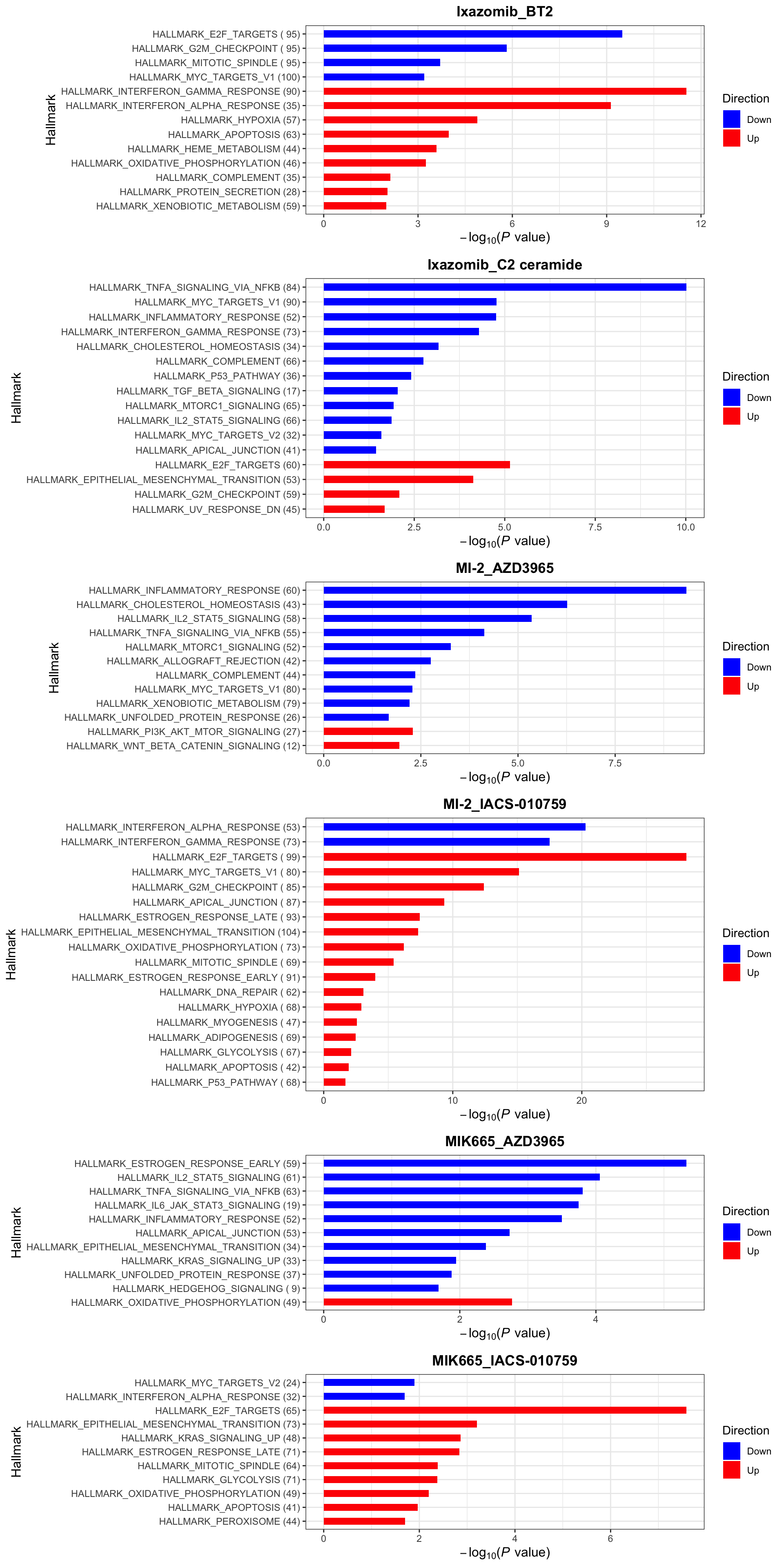

Note that since more negative CI scores indicate higher synergy, pathways labelled as Down are the pathways associated with higher synergy
If a combination is not shown here, it means there’s no significantly enriched pathways with indicated threshold

KEGG (10% FDR)

enrichres$KEGG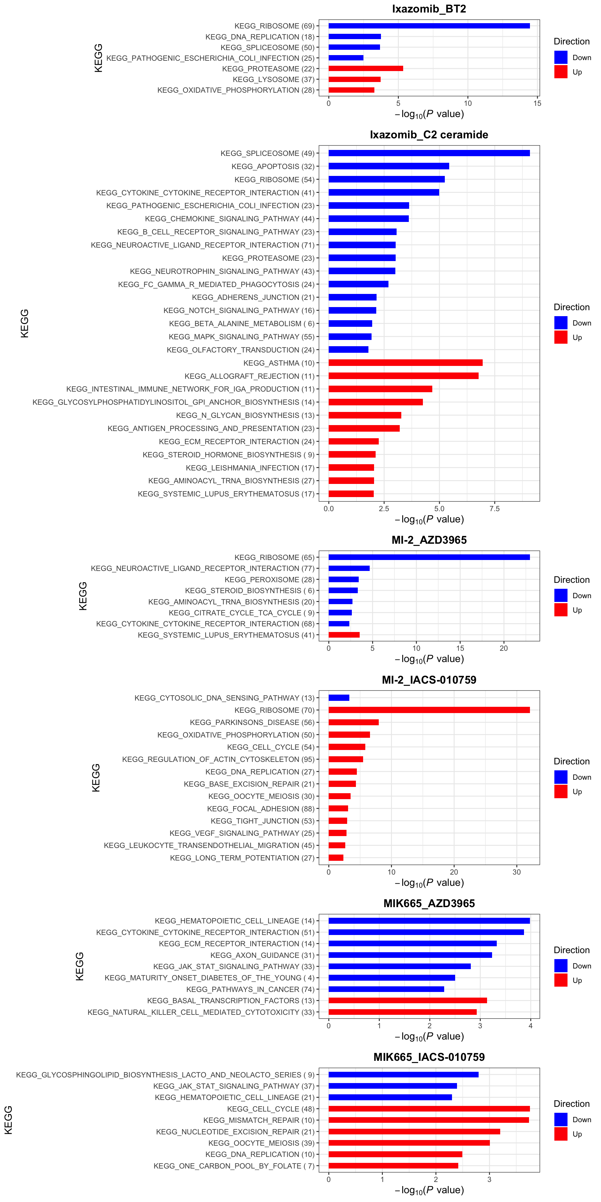

Note that since more negative CI scores indicate higher synergy, pathways labelled as Down are the pathways associated with higher synergy

Using Bayes synergy

Prepare list of selected synergy scores

synList <- bayesTabSum %>%
  mutate(combination = paste0(Drug_A, "_", Drug_B)) %>% 
  filter(combination %in% paste0(selectedPair$Drug_A,"_",selectedPair$Drug_B)) %>%
  mutate(score = syn)

Perform association tests

allRes <- predictSynergy(synList, exprMat)

P-value histogram

ggplot(allRes, aes(x=P.Value)) +
  geom_histogram() +
  facet_wrap(~combination)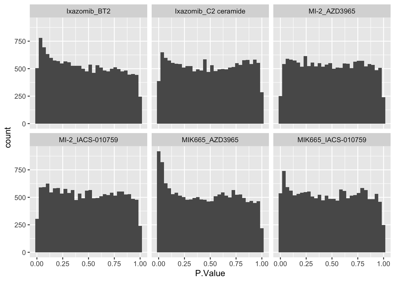

### Number of significant associations

Use 10% FDR (adj.P.Val < 0.1)

sumTab <- group_by(allRes, combination) %>%
  summarise(num = sum(adj.P.Val <= 0.10))
sumTab

# A tibble: 6 × 2
  combination            num
  <chr>                <int>
1 Ixazomib_BT2             0
2 Ixazomib_C2 ceramide     2
3 MI-2_AZD3965             0
4 MI-2_IACS-010759         0
5 MIK665_AZD3965         316
6 MIK665_IACS-010759       5

Use raw P.Value < 0.01 (without multiple hypothesis adjustment)

sumTab <- group_by(allRes, combination) %>%
  summarise(num = sum(P.Value <= 0.01))
sumTab

# A tibble: 6 × 2
  combination            num
  <chr>                <int>
1 Ixazomib_BT2           338
2 Ixazomib_C2 ceramide   218
3 MI-2_AZD3965           130
4 MI-2_IACS-010759       168
5 MIK665_AZD3965         714
6 MIK665_IACS-010759     371

List of significantly associated genes (raw P < 0.01)

allRes.sig <- filter(allRes, P.Value < 0.01) %>% 
  select(combination, symbol, logFC, P.Value, adj.P.Val) %>%
  mutate_if(is.numeric, formatC, digits=1)
DT::datatable(allRes.sig)

Pathway Enrichment analysis

gmts = list(Hallmark= "../data/gmts/h.all.v6.2.symbols.gmt",
            KEGG = "../data/gmts/c2.cp.kegg.v6.2.symbols.gmt")

enrichres <- performEnrichmentOnList(allRes, gmts, pCut = 0.1, ifFDR = TRUE)

Cancer Hallmark (10% FDR)

enrichres$Hallmark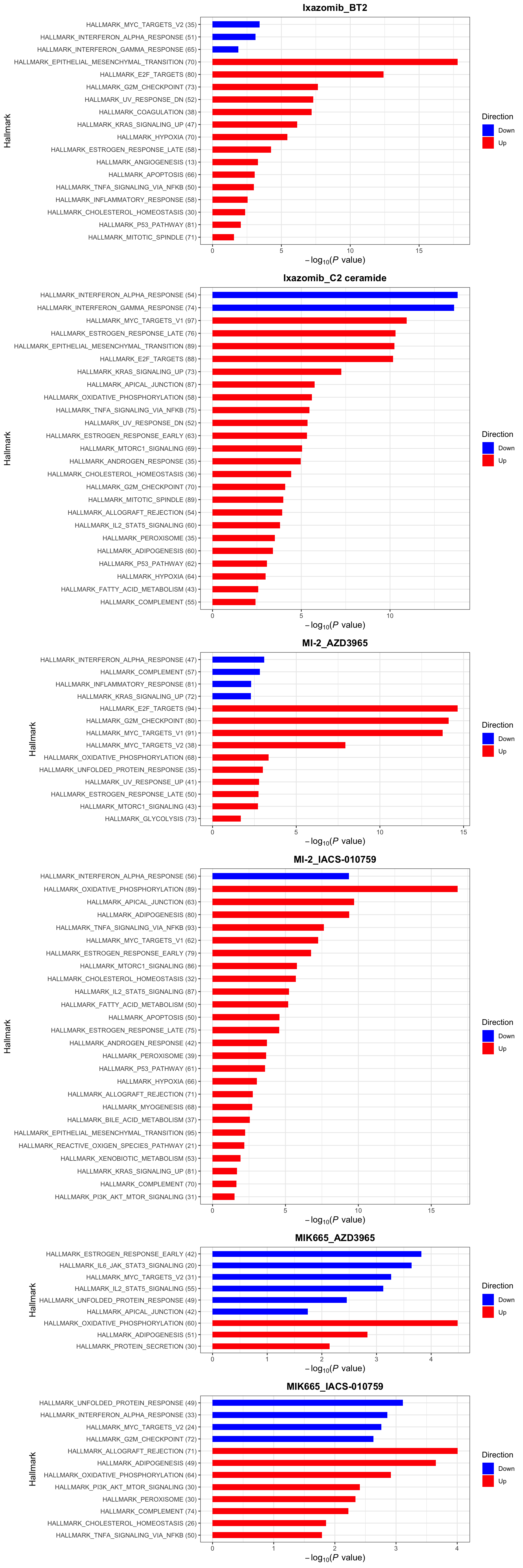

KEGG (10% FDR)

enrichres$KEGG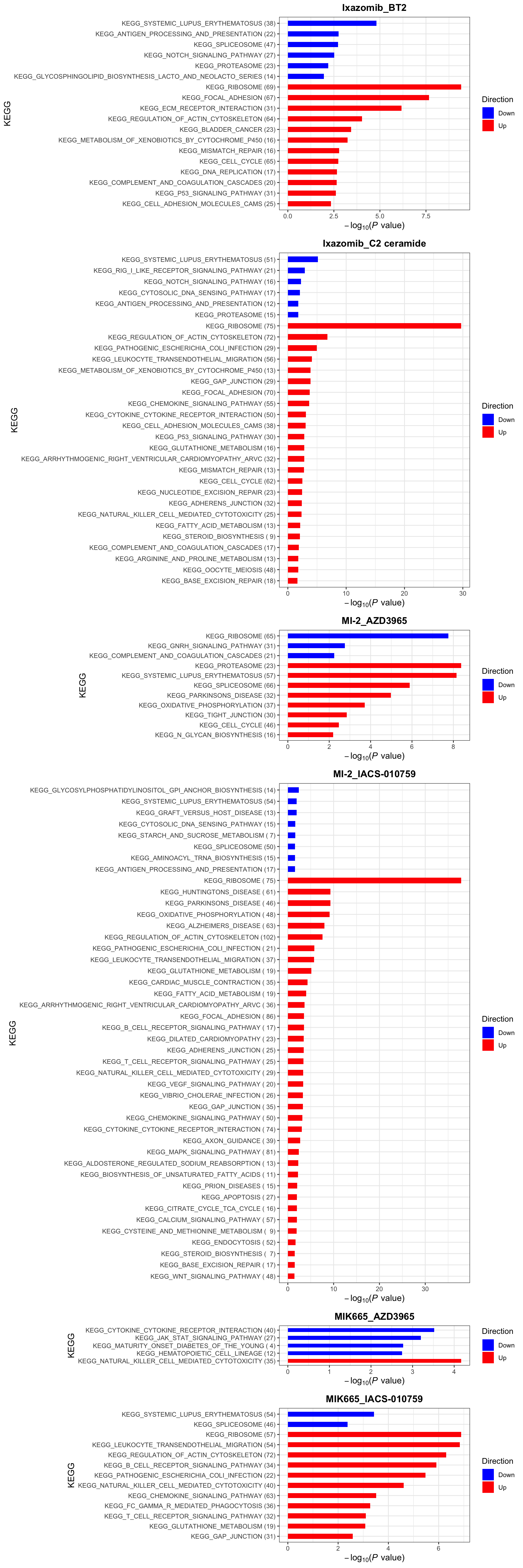

Explain synergy score by proteomics (from EMBL)

Processing proteomic data

Number of proteins and samples

load("../data/ProtWide.RData")
ProtWide <- ProtWide[,colnames(ProtWide) %in% unique(ciTabSum$Name)]
exprMat <- ProtWide
rownames(exprMat) <- getOneSymbol(rownames(exprMat), pos = "last", sep = "\\|")
#exprMat <- exprMat[!duplicated(rownames(exprMat)),]
dim(exprMat)

[1] 4873   23

Using Bliss synergy

Prepare list of selected synergy scores

synList <- ciTabSum %>%
  mutate(combination = paste0(Drug_A, "_", Drug_B)) %>% 
  filter(combination %in% paste0(selectedPair$Drug_A,"_",selectedPair$Drug_B)) %>%
  mutate(score = syn)

Perform association tests

allRes <- predictSynergy(synList, exprMat)

P-value histogram

ggplot(allRes, aes(x=P.Value)) +
  geom_histogram() +
  facet_wrap(~combination)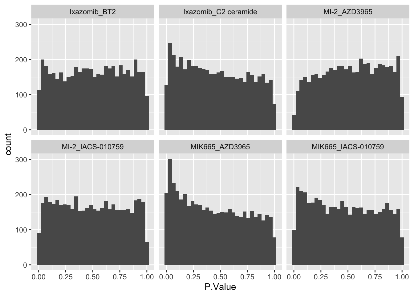

### Number of significant associations

Use 10% FDR (adj.P.Val < 0.1)

sumTab <- group_by(allRes, combination) %>%
  summarise(num = sum(adj.P.Val <= 0.10))
sumTab

# A tibble: 6 × 2
  combination            num
  <chr>                <int>
1 Ixazomib_BT2             2
2 Ixazomib_C2 ceramide     0
3 MI-2_AZD3965             0
4 MI-2_IACS-010759         0
5 MIK665_AZD3965           2
6 MIK665_IACS-010759       0

Use raw P.Value < 0.01 (without multiple hypothesis adjustment)

sumTab <- group_by(allRes, combination) %>%
  summarise(num = sum(P.Value <= 0.01))
sumTab

# A tibble: 6 × 2
  combination            num
  <chr>                <int>
1 Ixazomib_BT2            70
2 Ixazomib_C2 ceramide    61
3 MI-2_AZD3965            28
4 MI-2_IACS-010759        58
5 MIK665_AZD3965         129
6 MIK665_IACS-010759      56

List of significantly associated genes (raw P < 0.01)

allRes.sig <- filter(allRes, P.Value < 0.01) %>% 
  select(combination, symbol, logFC, P.Value, adj.P.Val) %>%
  mutate_if(is.numeric, formatC, digits=1)
DT::datatable(allRes.sig)

Pathway Enrichment analysis

gmts = list(Hallmark= "../data/gmts/h.all.v6.2.symbols.gmt",
            KEGG = "../data/gmts/c2.cp.kegg.v6.2.symbols.gmt")

enrichres <- performEnrichmentOnList(allRes, gmts, pCut = 0.1, ifFDR = TRUE)

[1] "No sets passed the criteria for MI-2_AZD3965 in KEGG"

Cancer Hallmark (10% FDR)

enrichres$Hallmark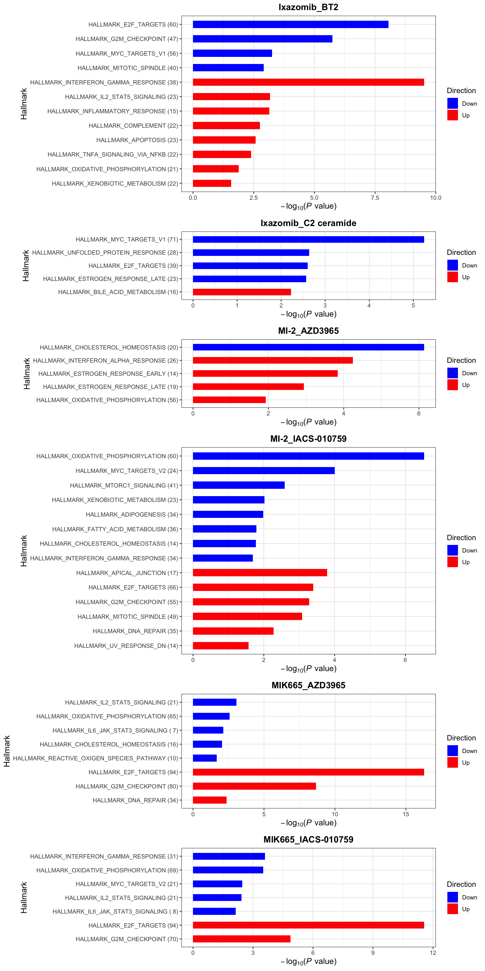

KEGG (10% FDR)

enrichres$KEGG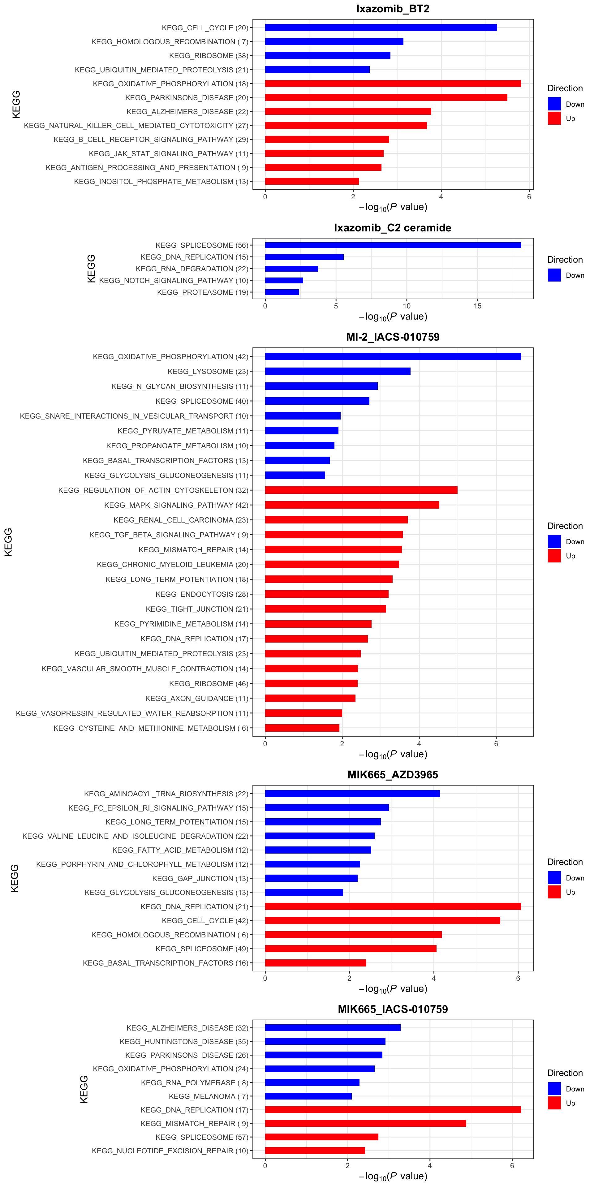

Using Bayes synergy

Prepare list of selected synergy scores

synList <- bayesTabSum %>%
  mutate(combination = paste0(Drug_A, "_", Drug_B)) %>% 
  filter(combination %in% paste0(selectedPair$Drug_A,"_",selectedPair$Drug_B)) %>%
  mutate(score = syn)

Perform association tests

allRes <- predictSynergy(synList, exprMat)

P-value histogram

ggplot(allRes, aes(x=P.Value)) +
  geom_histogram() +
  facet_wrap(~combination)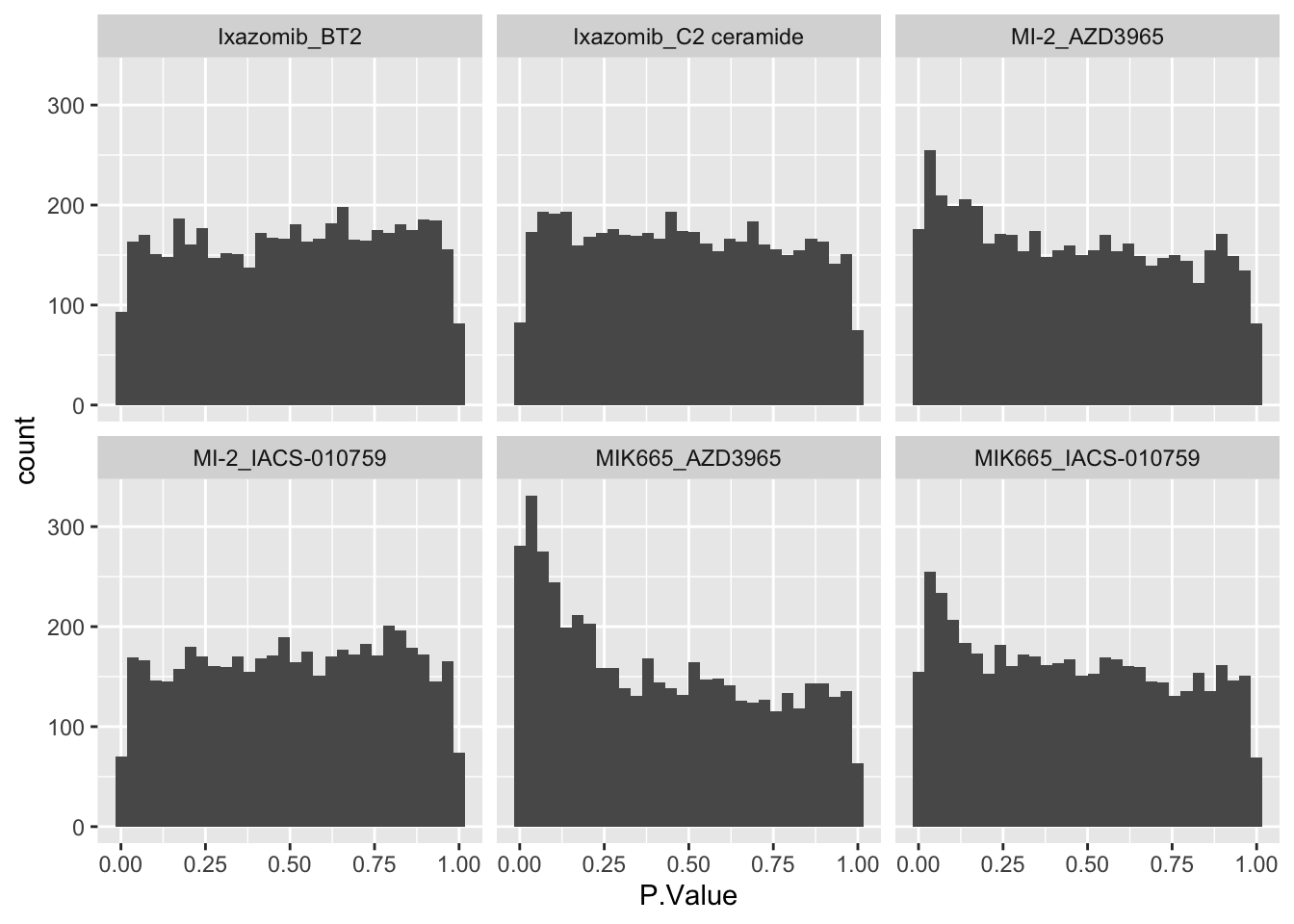

### Number of significant associations

Use 10% FDR (adj.P.Val < 0.1)

sumTab <- group_by(allRes, combination) %>%
  summarise(num = sum(adj.P.Val <= 0.10))
sumTab

# A tibble: 6 × 2
  combination            num
  <chr>                <int>
1 Ixazomib_BT2             2
2 Ixazomib_C2 ceramide     1
3 MI-2_AZD3965             0
4 MI-2_IACS-010759         0
5 MIK665_AZD3965           4
6 MIK665_IACS-010759       1

Use raw P.Value < 0.01 (without multiple hypothesis adjustment)

sumTab <- group_by(allRes, combination) %>%
  summarise(num = sum(P.Value <= 0.01))
sumTab

# A tibble: 6 × 2
  combination            num
  <chr>                <int>
1 Ixazomib_BT2            53
2 Ixazomib_C2 ceramide    45
3 MI-2_AZD3965           121
4 MI-2_IACS-010759        40
5 MIK665_AZD3965         180
6 MIK665_IACS-010759      98

List of significantly associated genes (raw P < 0.01)

allRes.sig <- filter(allRes, P.Value < 0.01) %>% 
  select(combination, symbol, logFC, P.Value, adj.P.Val) %>%
  mutate_if(is.numeric, formatC, digits=1)
DT::datatable(allRes.sig)

Pathway Enrichment analysis

gmts = list(Hallmark= "../data/gmts/h.all.v6.2.symbols.gmt",
            KEGG = "../data/gmts/c2.cp.kegg.v6.2.symbols.gmt")

enrichres <- performEnrichmentOnList(allRes, gmts, pCut = 0.1, ifFDR = TRUE)

Cancer Hallmark (10% FDR)

enrichres$Hallmark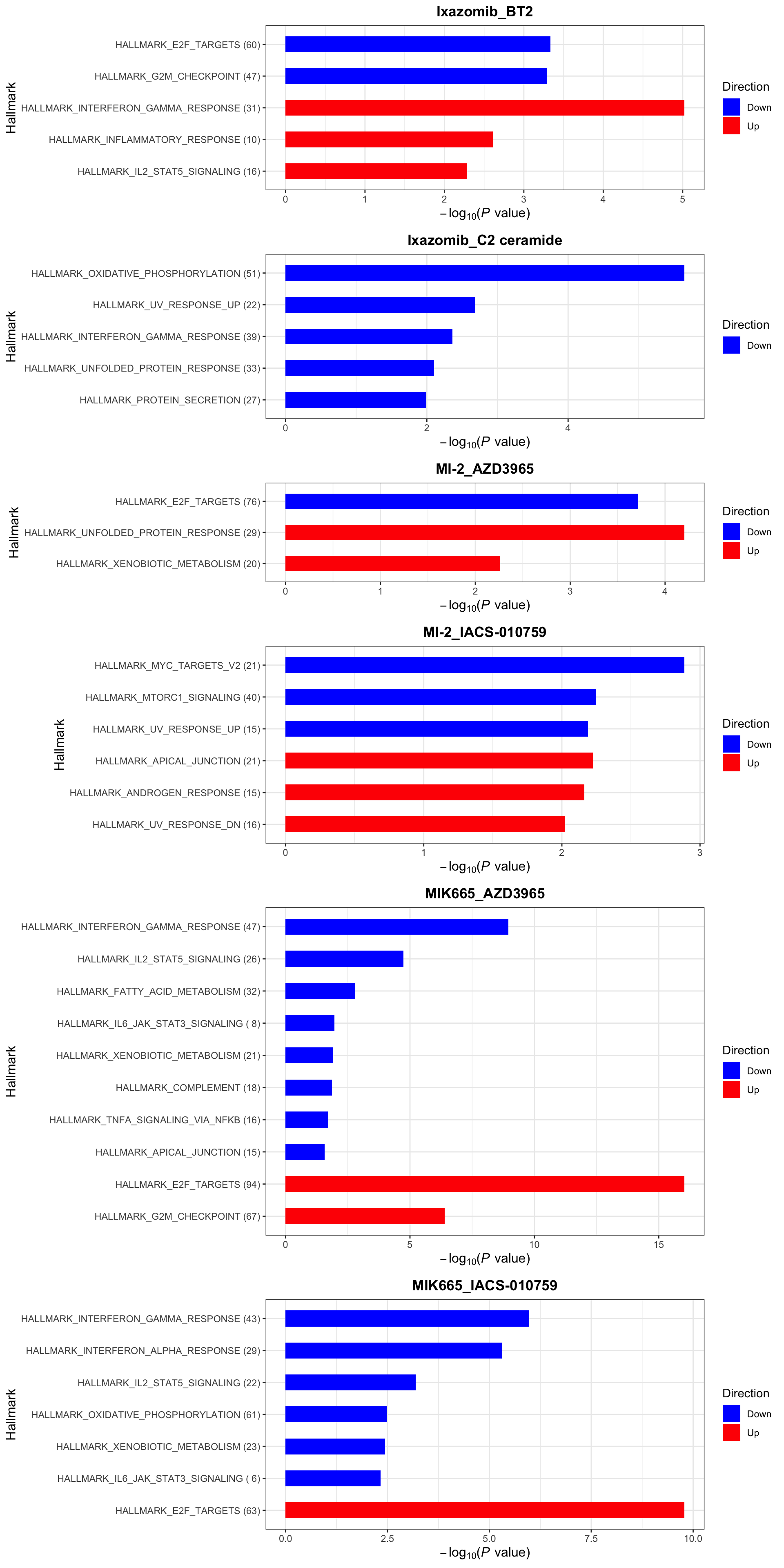

KEGG (10% FDR)

enrichres$KEGG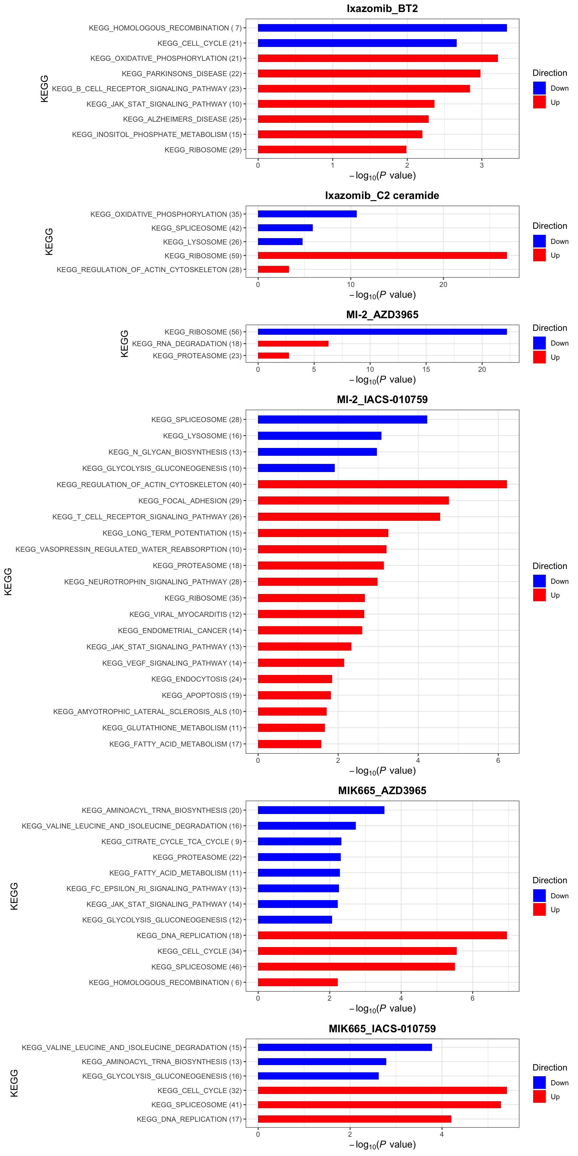

Explain synergy score by proteomics (from AG Krijgsveld)

Processing proteomic data

library(SummarizedExperiment)


protData <- readRDS("../data/SC005_SummarizedExperiment_proteomics.RDS")
#select baseline samples
protData <- protData[!rowData(protData)$Gene_name %in% c("",NA), protData$cell.line %in% unique(ciTabSum$Name) & protData$condition == "U"]
rowData(protData)$Gene_name <- getOneSymbol(rowData(protData)$Gene_name, pos = "first")
assayNames(protData) <- "norm"
protTab <- jyluMisc::sumToTidy(protData) %>%
  group_by(cell.line, Gene_name) %>%
  summarise(count = mean(norm, na.rm=TRUE)) %>%
  dplyr::rename(symbol = Gene_name, cellLine = cell.line) %>%
  mutate(colID = cellLine) %>%
  ungroup()

protData <- jyluMisc::tidyToSum(protTab, rowID = "symbol", colID = "colID", 
                     values = "count", annoRow = "symbol", 
                     annoCol = c("cellLine"))

exprMat <- assay(protData)
#rownames(exprMat) <- rowData(protData)$symbol

dim(exprMat)

[1] 2640   11

Using Bliss synergy

Prepare list of selected synergy scores

synList <- ciTabSum %>%
  mutate(combination = paste0(Drug_A, "_", Drug_B)) %>% 
  filter(combination %in% paste0(selectedPair$Drug_A,"_",selectedPair$Drug_B)) %>%
  mutate(score = syn)

Perform association tests

allRes <- predictSynergy(synList, exprMat)

P-value histogram

ggplot(allRes, aes(x=P.Value)) +
  geom_histogram() +
  facet_wrap(~combination)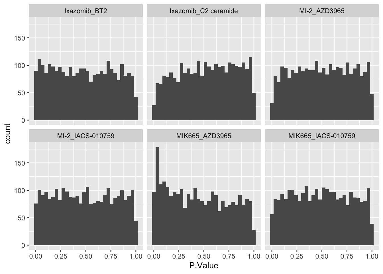

### Number of significant associations

Use 10% FDR (adj.P.Val < 0.1)

sumTab <- group_by(allRes, combination) %>%
  summarise(num = sum(adj.P.Val <= 0.10))
sumTab

# A tibble: 6 × 2
  combination            num
  <chr>                <int>
1 Ixazomib_BT2            15
2 Ixazomib_C2 ceramide     0
3 MI-2_AZD3965             0
4 MI-2_IACS-010759         1
5 MIK665_AZD3965           1
6 MIK665_IACS-010759       0

Use raw P.Value < 0.01 (without multiple hypothesis adjustment)

sumTab <- group_by(allRes, combination) %>%
  summarise(num = sum(P.Value <= 0.01))
sumTab

# A tibble: 6 × 2
  combination            num
  <chr>                <int>
1 Ixazomib_BT2            60
2 Ixazomib_C2 ceramide    11
3 MI-2_AZD3965            16
4 MI-2_IACS-010759        47
5 MIK665_AZD3965          74
6 MIK665_IACS-010759      37

List of significantly associated genes (raw P < 0.01)

allRes.sig <- filter(allRes, P.Value < 0.01) %>% 
  select(combination, symbol, logFC, P.Value, adj.P.Val) %>%
  mutate_if(is.numeric, formatC, digits=1)
DT::datatable(allRes.sig)

Pathway Enrichment analysis

gmts = list(Hallmark= "../data/gmts/h.all.v6.2.symbols.gmt",
            KEGG = "../data/gmts/c2.cp.kegg.v6.2.symbols.gmt")

enrichres <- performEnrichmentOnList(allRes, gmts, pCut = 0.1, ifFDR = TRUE)

[1] "No sets passed the criteria for Ixazomib_C2 ceramide in Hallmark"

Cancer Hallmark (10% FDR)

enrichres$Hallmark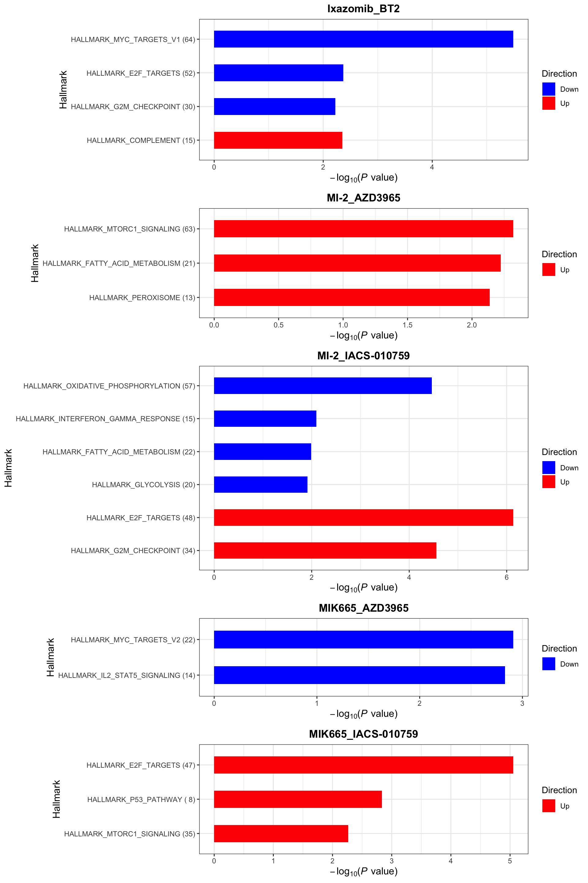

KEGG (10% FDR)

enrichres$KEGG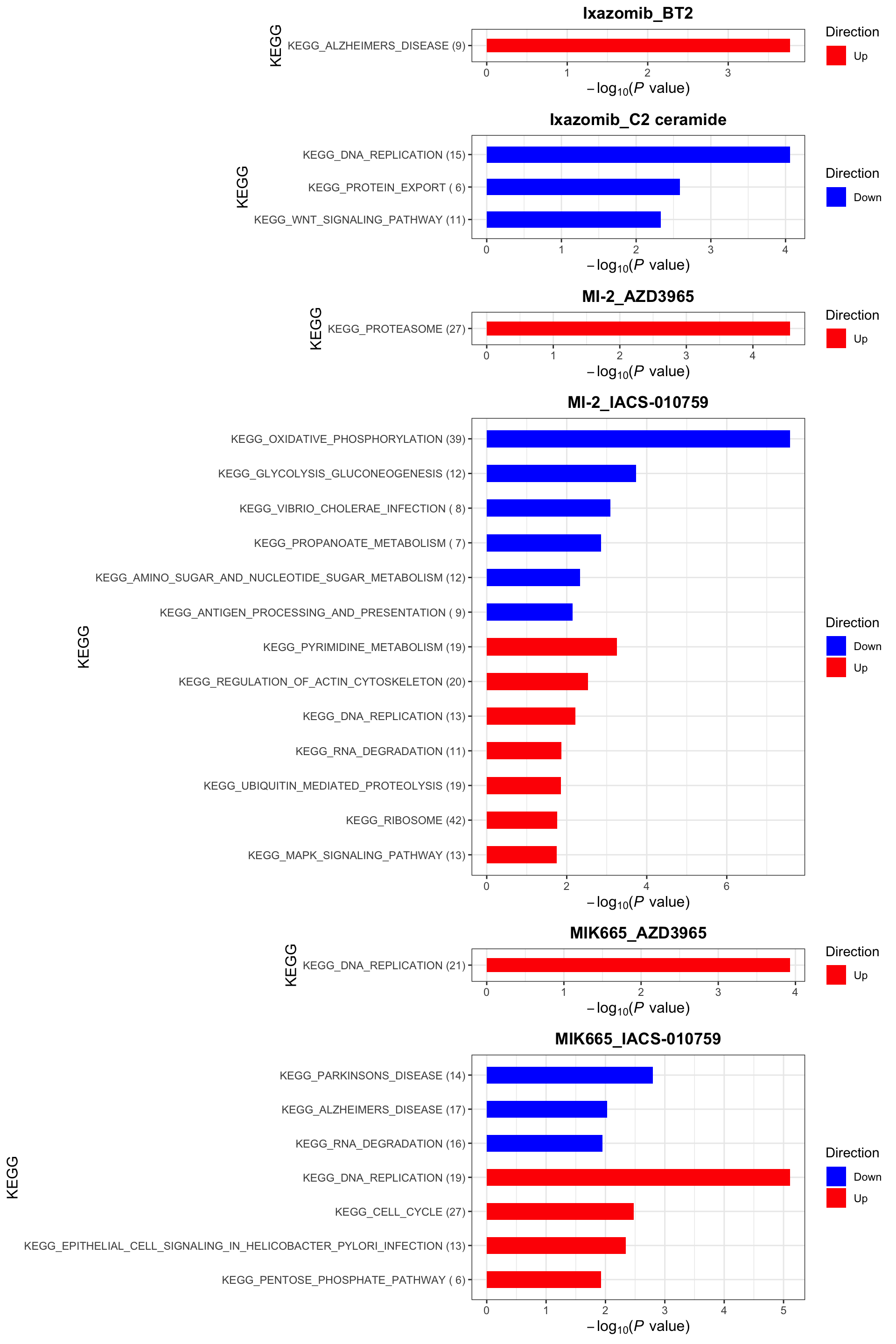

Using Bayes synergy

Prepare list of selected synergy scores

synList <- bayesTabSum %>%
  mutate(combination = paste0(Drug_A, "_", Drug_B)) %>% 
  filter(combination %in% paste0(selectedPair$Drug_A,"_",selectedPair$Drug_B)) %>%
  mutate(score = syn)

Perform association tests

allRes <- predictSynergy(synList, exprMat)

P-value histogram

ggplot(allRes, aes(x=P.Value)) +
  geom_histogram() +
  facet_wrap(~combination)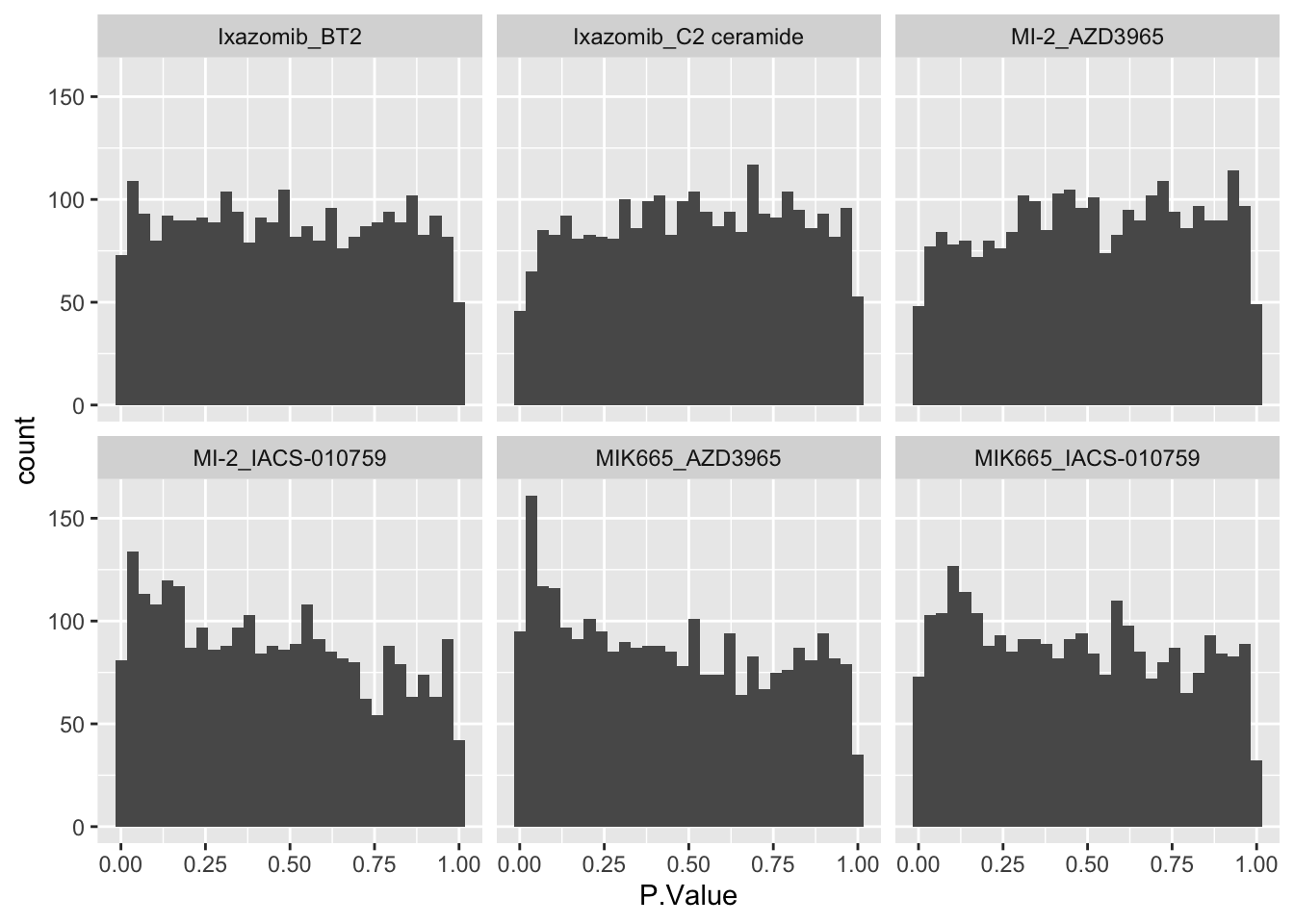

### Number of significant associations

Use 10% FDR (adj.P.Val < 0.1)

sumTab <- group_by(allRes, combination) %>%
  summarise(num = sum(adj.P.Val <= 0.10))
sumTab

# A tibble: 6 × 2
  combination            num
  <chr>                <int>
1 Ixazomib_BT2             3
2 Ixazomib_C2 ceramide     0
3 MI-2_AZD3965             0
4 MI-2_IACS-010759         0
5 MIK665_AZD3965           2
6 MIK665_IACS-010759       1

Use raw P.Value < 0.01 (without multiple hypothesis adjustment)

sumTab <- group_by(allRes, combination) %>%
  summarise(num = sum(P.Value <= 0.01))
sumTab

# A tibble: 6 × 2
  combination            num
  <chr>                <int>
1 Ixazomib_BT2            55
2 Ixazomib_C2 ceramide    25
3 MI-2_AZD3965            28
4 MI-2_IACS-010759        50
5 MIK665_AZD3965          60
6 MIK665_IACS-010759      50

List of significantly associated genes (raw P < 0.01)

allRes.sig <- filter(allRes, P.Value < 0.01) %>% 
  select(combination, symbol, logFC, P.Value, adj.P.Val) %>%
  mutate_if(is.numeric, formatC, digits=1)
DT::datatable(allRes.sig)

Pathway Enrichment analysis

gmts = list(Hallmark= "../data/gmts/h.all.v6.2.symbols.gmt",
            KEGG = "../data/gmts/c2.cp.kegg.v6.2.symbols.gmt")

enrichres <- performEnrichmentOnList(allRes, gmts, pCut = 0.1, ifFDR = TRUE)

[1] "No sets passed the criteria for MI-2_AZD3965 in Hallmark"
[1] "No sets passed the criteria for MI-2_IACS-010759 in Hallmark"
[1] "No sets passed the criteria for Ixazomib_BT2 in KEGG"

Cancer Hallmark (10% FDR)

enrichres$Hallmark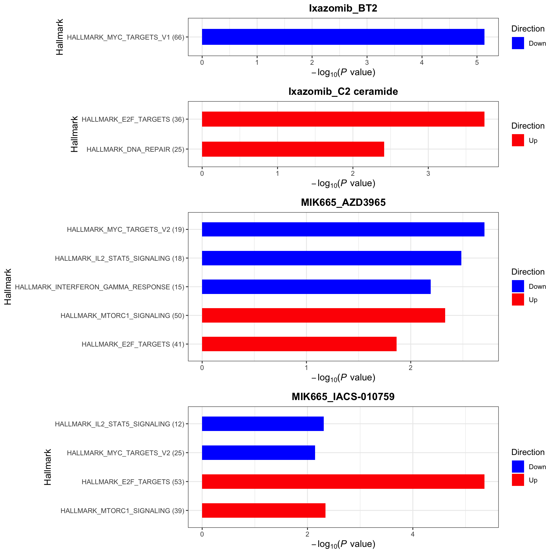

KEGG (10% FDR)

enrichres$KEGG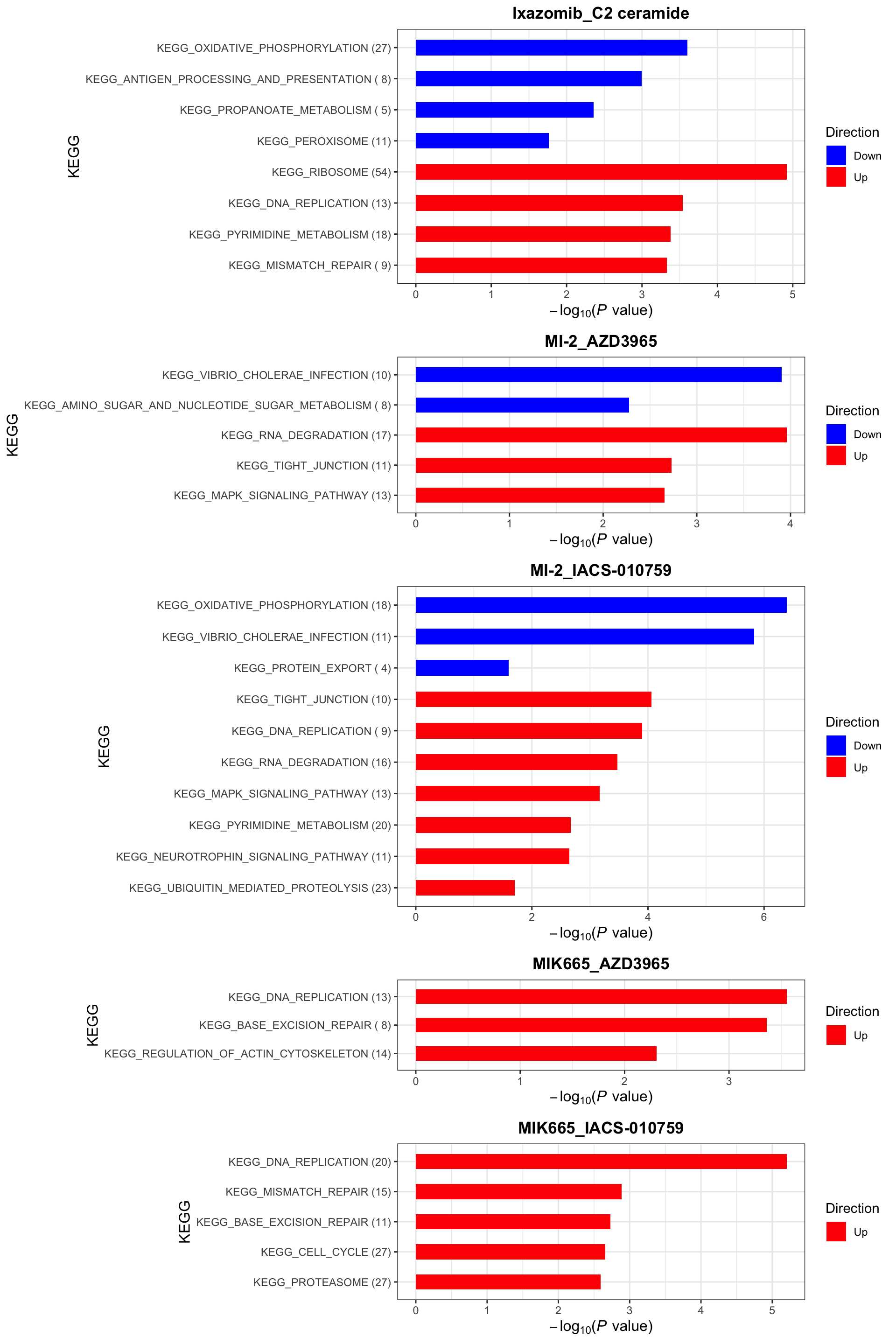

sessionInfo()

R version 4.2.0 (2022-04-22)
Platform: x86_64-apple-darwin17.0 (64-bit)
Running under: macOS Big Sur/Monterey 10.16

Matrix products: default
BLAS:   /Library/Frameworks/R.framework/Versions/4.2/Resources/lib/libRblas.0.dylib
LAPACK: /Library/Frameworks/R.framework/Versions/4.2/Resources/lib/libRlapack.dylib

locale:
[1] en_US.UTF-8/en_US.UTF-8/en_US.UTF-8/C/en_US.UTF-8/en_US.UTF-8

attached base packages:
[1] stats4    stats     graphics  grDevices utils     datasets  methods  
[8] base     

other attached packages:
 [1] SummarizedExperiment_1.26.1 Biobase_2.56.0             
 [3] GenomicRanges_1.48.0        GenomeInfoDb_1.32.2        
 [5] IRanges_2.30.0              S4Vectors_0.34.0           
 [7] BiocGenerics_0.42.0         MatrixGenerics_1.8.1       
 [9] matrixStats_0.62.0          gridExtra_2.3              
[11] forcats_0.5.1               stringr_1.4.1              
[13] dplyr_1.0.9                 purrr_0.3.4                
[15] readr_2.1.2                 tidyr_1.2.0                
[17] tibble_3.1.8                ggplot2_3.4.1              
[19] tidyverse_1.3.2            

loaded via a namespace (and not attached):
  [1] readxl_1.4.0           backports_1.4.1        fastmatch_1.1-3       
  [4] drc_3.0-1              jyluMisc_0.1.5         workflowr_1.7.0       
  [7] igraph_1.3.4           shinydashboard_0.7.2   splines_4.2.0         
 [10] crosstalk_1.2.0        BiocParallel_1.30.3    TH.data_1.1-1         
 [13] digest_0.6.30          htmltools_0.5.4        fansi_1.0.3           
 [16] magrittr_2.0.3         googlesheets4_1.0.0    cluster_2.1.3         
 [19] tzdb_0.3.0             limma_3.52.2           modelr_0.1.8          
 [22] sandwich_3.0-2         piano_2.12.0           colorspace_2.0-3      
 [25] ggrepel_0.9.1          rvest_1.0.2            haven_2.5.0           
 [28] xfun_0.31              crayon_1.5.2           RCurl_1.98-1.7        
 [31] jsonlite_1.8.3         survival_3.4-0         zoo_1.8-10            
 [34] glue_1.6.2             survminer_0.4.9        gtable_0.3.0          
 [37] gargle_1.2.0           zlibbioc_1.42.0        XVector_0.36.0        
 [40] DelayedArray_0.22.0    car_3.1-0              abind_1.4-5           
 [43] scales_1.2.0           vsn_3.64.0             mvtnorm_1.1-3         
 [46] DBI_1.1.3              relations_0.6-12       rstatix_0.7.0         
 [49] Rcpp_1.0.9             plotrix_3.8-2          xtable_1.8-4          
 [52] preprocessCore_1.58.0  km.ci_0.5-6            DT_0.23               
 [55] htmlwidgets_1.5.4      httr_1.4.3             fgsea_1.22.0          
 [58] gplots_3.1.3           ellipsis_0.3.2         pkgconfig_2.0.3       
 [61] farver_2.1.1           sass_0.4.2             dbplyr_2.2.1          
 [64] utf8_1.2.2             labeling_0.4.2         tidyselect_1.1.2      
 [67] rlang_1.0.6            later_1.3.0            munsell_0.5.0         
 [70] cellranger_1.1.0       tools_4.2.0            visNetwork_2.1.0      
 [73] cachem_1.0.6           cli_3.4.1              generics_0.1.3        
 [76] broom_1.0.0            evaluate_0.15          fastmap_1.1.0         
 [79] yaml_2.3.5             knitr_1.39             fs_1.5.2              
 [82] survMisc_0.5.6         caTools_1.18.2         nlme_3.1-158          
 [85] mime_0.12              slam_0.1-50            xml2_1.3.3            
 [88] compiler_4.2.0         rstudioapi_0.13        affyio_1.66.0         
 [91] ggsignif_0.6.3         marray_1.74.0          reprex_2.0.1          
 [94] bslib_0.4.1            stringi_1.7.8          highr_0.9             
 [97] lattice_0.20-45        Matrix_1.5-4           KMsurv_0.1-5          
[100] shinyjs_2.1.0          vctrs_0.5.2            pillar_1.8.0          
[103] lifecycle_1.0.3        BiocManager_1.30.18    jquerylib_0.1.4       
[106] data.table_1.14.8      cowplot_1.1.1          bitops_1.0-7          
[109] httpuv_1.6.6           affy_1.74.0            R6_2.5.1              
[112] promises_1.2.0.1       KernSmooth_2.23-20     codetools_0.2-18      
[115] MASS_7.3-58            gtools_3.9.3           exactRankTests_0.8-35 
[118] assertthat_0.2.1       rprojroot_2.0.3        withr_2.5.0           
[121] multcomp_1.4-19        GenomeInfoDbData_1.2.8 mgcv_1.8-40           
[124] parallel_4.2.0         hms_1.1.1              grid_4.2.0            
[127] rmarkdown_2.14         carData_3.0-5          googledrive_2.0.0     
[130] git2r_0.30.1           maxstat_0.7-25         ggpubr_0.4.0          
[133] sets_1.0-21            shiny_1.7.4            lubridate_1.8.0

Analysis of combinatorial effect using simple bliss model

Junyan Lu

2022-04-25

Load libraries and datasets

Calculate CI for the combination of bases and combi drugs

Visualize CI for each drug and concentration

Summarise CI

Visualization of synergistic and antagoistic effect

Scatter plot

Matrix visualization

Dose-response plots for synergistic effect

Test for synergistic effect related to genomics (SNVs)

Boxplots for associations passed p.adj < 0.25

Correlate combination effect with clinical drug responses

Test per concentration

P-value histogram per clinical drug

Correlation coefficient distribution

P-value heatmap

Scatter plot of significant associations

Top 20 negative associations: higher resistance correlated with lower CI (more synergistic)

Top 9 positive associations: higher resistance correlated with higher CI (more antagonistic)

At summarised level

Calculate AUC for clinical drugs

Correlate AUC with summarised CI

P-value histogram per clinical drug

Correlation coefficient distribution

P-value heatmap

Scatter plot of significant associations

Top 20 negative associations with synergy: higher resistance correlated with higher synergy

Top 20 positive associations with antagonistic: higher resistance correlated with more antagonistic effect

Define non-responder cell lines and test for synergy

Define non-responders to clinical drugs using the mirror method proposed by Wolfgang

Plot response distribution for each clinical drug

Comapre BayeSynergy score with Bliss synergy score

Overall comparison

Visualize per cellline + clinical drug

Multi-variate regression to identfy associations between genomics and synergy

Bliss synergy

Variance explained (R2) for each selected synergy by genomics

Genes that can explain synergy in multi-variate models (for selected drug pairs)

Genes that can explain synergy in multi-variate models (for all drug pairs)

Bayes synergy

Variance explained (R2) for each selected synergy by genomics

Genes that can explain synergy in multi-variate models (for selected drug pairs)

Genes that can explain synergy in multi-variate models (for all drug pairs)

Explain synergy score by transcriptomics

Processing transcriptomic data

Using Bliss synergy

Prepare list of selected synergy scores

Perform association tests

P-value histogram

Number of significant associations

Use 10% FDR (adj.P.Val < 0.1)

Use raw P.Value < 0.01 (without multiple hypothesis adjustment)

List of significantly associated genes (raw P < 0.01)

Pathway Enrichment analysis

Cancer Hallmark (10% FDR)

KEGG (10% FDR)

Using Bayes synergy

Prepare list of selected synergy scores

Perform association tests

P-value histogram

Use 10% FDR (adj.P.Val < 0.1)

Use raw P.Value < 0.01 (without multiple hypothesis adjustment)

List of significantly associated genes (raw P < 0.01)

Pathway Enrichment analysis

Cancer Hallmark (10% FDR)

KEGG (10% FDR)

Explain synergy score by proteomics (from EMBL)

Processing proteomic data

Using Bliss synergy

Prepare list of selected synergy scores

Perform association tests

P-value histogram

Use 10% FDR (adj.P.Val < 0.1)

Use raw P.Value < 0.01 (without multiple hypothesis adjustment)

List of significantly associated genes (raw P < 0.01)

Pathway Enrichment analysis

Cancer Hallmark (10% FDR)

KEGG (10% FDR)