Identify drug responses associated with genomics in CLL with IC50 screen data
Junyan Lu
9 June 2022
Last updated: 2022-06-09
Checks: 6 1
Knit directory: EMBL2016/analysis/
This reproducible R Markdown analysis was created with workflowr (version 1.7.0). The Checks tab describes the reproducibility checks that were applied when the results were created. The Past versions tab lists the development history.
The R Markdown is untracked by Git. To know which version of the R
Markdown file created these results, you’ll want to first commit it to
the Git repo. If you’re still working on the analysis, you can ignore
this warning. When you’re finished, you can run
wflow_publish to commit the R Markdown file and build the
HTML.
Great job! The global environment was empty. Objects defined in the global environment can affect the analysis in your R Markdown file in unknown ways. For reproduciblity it’s best to always run the code in an empty environment.
The command set.seed(20210512) was run prior to running
the code in the R Markdown file. Setting a seed ensures that any results
that rely on randomness, e.g. subsampling or permutations, are
reproducible.
Great job! Recording the operating system, R version, and package versions is critical for reproducibility.
Nice! There were no cached chunks for this analysis, so you can be confident that you successfully produced the results during this run.
Great job! Using relative paths to the files within your workflowr project makes it easier to run your code on other machines.
Great! You are using Git for version control. Tracking code development and connecting the code version to the results is critical for reproducibility.
The results in this page were generated with repository version 12d1722. See the Past versions tab to see a history of the changes made to the R Markdown and HTML files.
Note that you need to be careful to ensure that all relevant files for
the analysis have been committed to Git prior to generating the results
(you can use wflow_publish or
wflow_git_commit). workflowr only checks the R Markdown
file, but you know if there are other scripts or data files that it
depends on. Below is the status of the Git repository when the results
were generated:
Ignored files:
    Ignored:    .DS_Store
    Ignored:    .Rhistory
    Ignored:    analysis/.DS_Store
    Ignored:    analysis/.Rhistory
    Ignored:    analysis/CDK_analysis_cache/
    Ignored:    analysis/boxplot_AUC.png
    Ignored:    analysis/consensus_clustering_CPS_cache/
    Ignored:    analysis/consensus_clustering_noFit_cache/
    Ignored:    analysis/dose_curve.png
    Ignored:    analysis/targetDist.png
    Ignored:    analysis/toxivity_box.png
    Ignored:    analysis/volcano.png
    Ignored:    data/.DS_Store
    Ignored:    output/.DS_Store

Untracked files:
    Untracked:  analysis/AUC_CLL_IC50/
    Untracked:  analysis/BRAF_analysis.Rmd
    Untracked:  analysis/CDK_analysis.Rmd
    Untracked:  analysis/GSVA_analysis.Rmd
    Untracked:  analysis/NOTCH1_signature.Rmd
    Untracked:  analysis/autoluminescence.Rmd
    Untracked:  analysis/bar_plot_mixed.pdf
    Untracked:  analysis/bar_plot_mixed_noU1.pdf
    Untracked:  analysis/beatAML/
    Untracked:  analysis/cohortComposition_CLLsamples.pdf
    Untracked:  analysis/cohortComposition_allSamples.pdf
    Untracked:  analysis/consensus_clustering.Rmd
    Untracked:  analysis/consensus_clustering_CPS.Rmd
    Untracked:  analysis/consensus_clustering_IC50.Rmd
    Untracked:  analysis/consensus_clustering_beatAML.Rmd
    Untracked:  analysis/consensus_clustering_noFit.Rmd
    Untracked:  analysis/consensus_clusters.pdf
    Untracked:  analysis/disease_specific.Rmd
    Untracked:  analysis/dose_curve_selected.pdf
    Untracked:  analysis/drugScreens_reproducibility.Rmd
    Untracked:  analysis/genomic_association.Rmd
    Untracked:  analysis/genomic_association_IC50.Rmd
    Untracked:  analysis/genomic_association_allDisease.Rmd
    Untracked:  analysis/mean_autoluminescence_val.csv
    Untracked:  analysis/mean_autoluminescence_val.xlsx
    Untracked:  analysis/noFit_CLL/
    Untracked:  analysis/number_associations.pdf
    Untracked:  analysis/overview.Rmd
    Untracked:  analysis/plotCohort.Rmd
    Untracked:  analysis/preprocess.Rmd
    Untracked:  analysis/volcano_noBlocking.pdf
    Untracked:  code/utils.R
    Untracked:  data/BeatAML_Waves1_2/
    Untracked:  data/ic50Tab.RData
    Untracked:  data/newEMBL_20210806.RData
    Untracked:  data/patMeta.RData
    Untracked:  data/targetAnnotation_all.csv
    Untracked:  output/gene_associations/
    Untracked:  output/resConsClust.RData
    Untracked:  output/resConsClust_aucFit.RData
    Untracked:  output/resConsClust_beatAML.RData
    Untracked:  output/resConsClust_cps.RData
    Untracked:  output/resConsClust_ic50.RData
    Untracked:  output/resConsClust_noFit.RData
    Untracked:  output/screenData.RData

Unstaged changes:
    Modified:   _workflowr.yml
    Modified:   analysis/_site.yml
    Deleted:    analysis/about.Rmd
    Modified:   analysis/index.Rmd
    Deleted:    analysis/license.Rmd
Note that any generated files, e.g. HTML, png, CSS, etc., are not included in this status report because it is ok for generated content to have uncommitted changes.
There are no past versions. Publish this analysis with
wflow_publish() to start tracking its development.
Load libraries and dataset
Load datasets
Preprocessing IC50 screen data
Select CLL samples and use AUC as measures of drug effect
screenData <- ic50 %>%
    dplyr::rename(viab = normVal, viab.auc  = normVal_auc, conc = Concentration) %>%
    filter(!Drug%in% c("PBS","DMSO"))

#for the drugs that are also in EMBL2016 screen, use the same name as in EMBL2016 screen
screenData <- mutate(screenData, emblName = targetAnno[match(Drug, targetAnno$nameIC50),]$nameEMBL2016) %>%
    mutate(Drug = ifelse(is.na(emblName), Drug, emblName)) %>%
    select(-emblName)
Overview of associations between drug responses and genomics in CLL
Using AUC of trepazoidal rule
Without blocking for IGHV
Only mutations occcured at least 5 times will be included in the test
Perform test
Adjust p-value use IHW, using standard deviation as covariate
meanSdTab <- tibble(name = rownames(viabMat),
                    meanVal = rowMeans(viabMat, na.rm = TRUE),
                    sdVal = genefilter::rowSds(viabMat, na.rm=TRUE))


ihwTab <- tibble(pval = pTab$p, name = pTab$drug) %>%
  left_join(meanSdTab)
ihwRes <- ihw(pval ~ sdVal,  data = ihwTab, alpha = 0.1)
pTab$p.adj.ihw <- adj_pvalues(ihwRes)
#plot(ihwRes)
Write out test result table
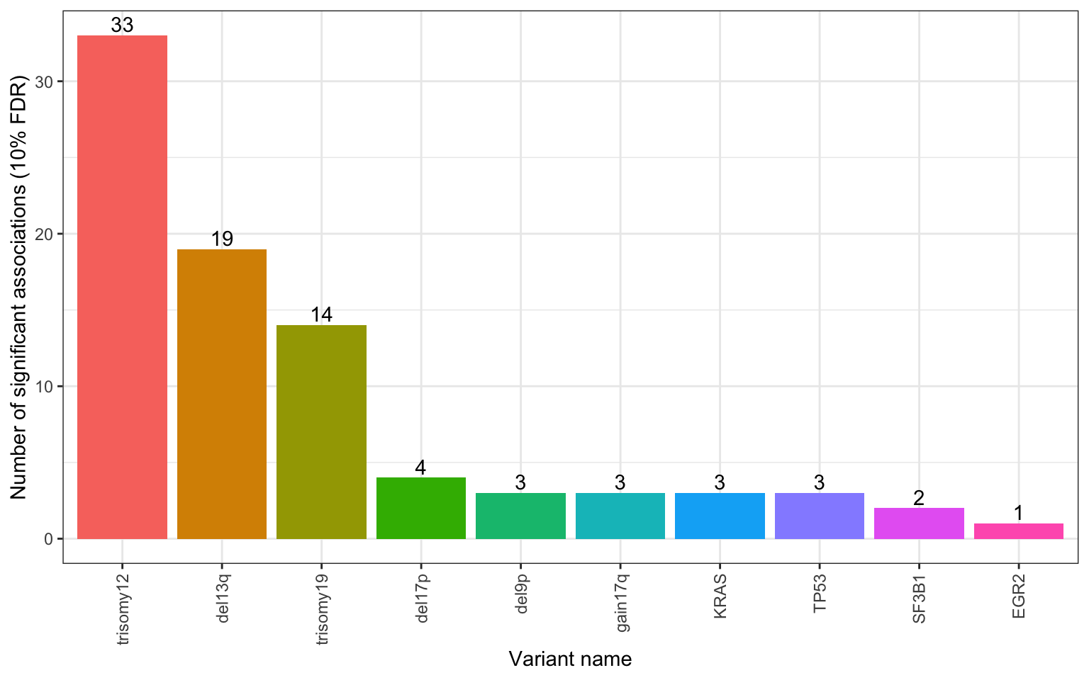
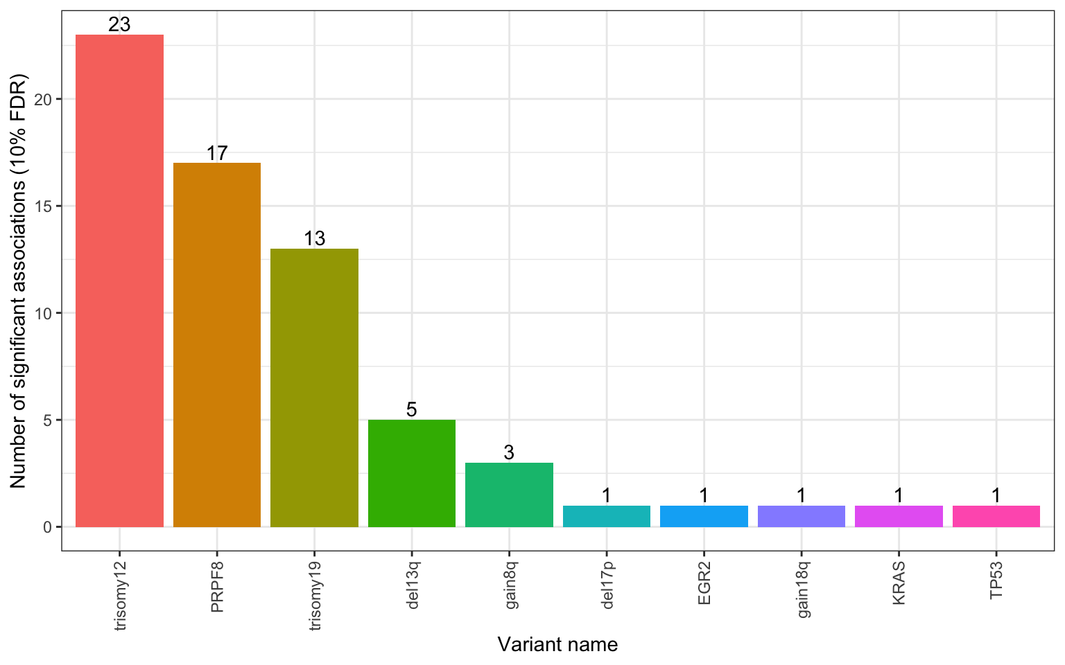
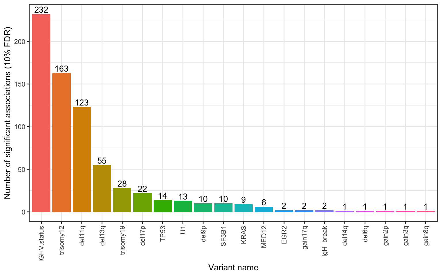
write_csv2(pTab,"../docs/p_table_noBlock_IC50.csv")Number of significant associations per gene (10% FDR)
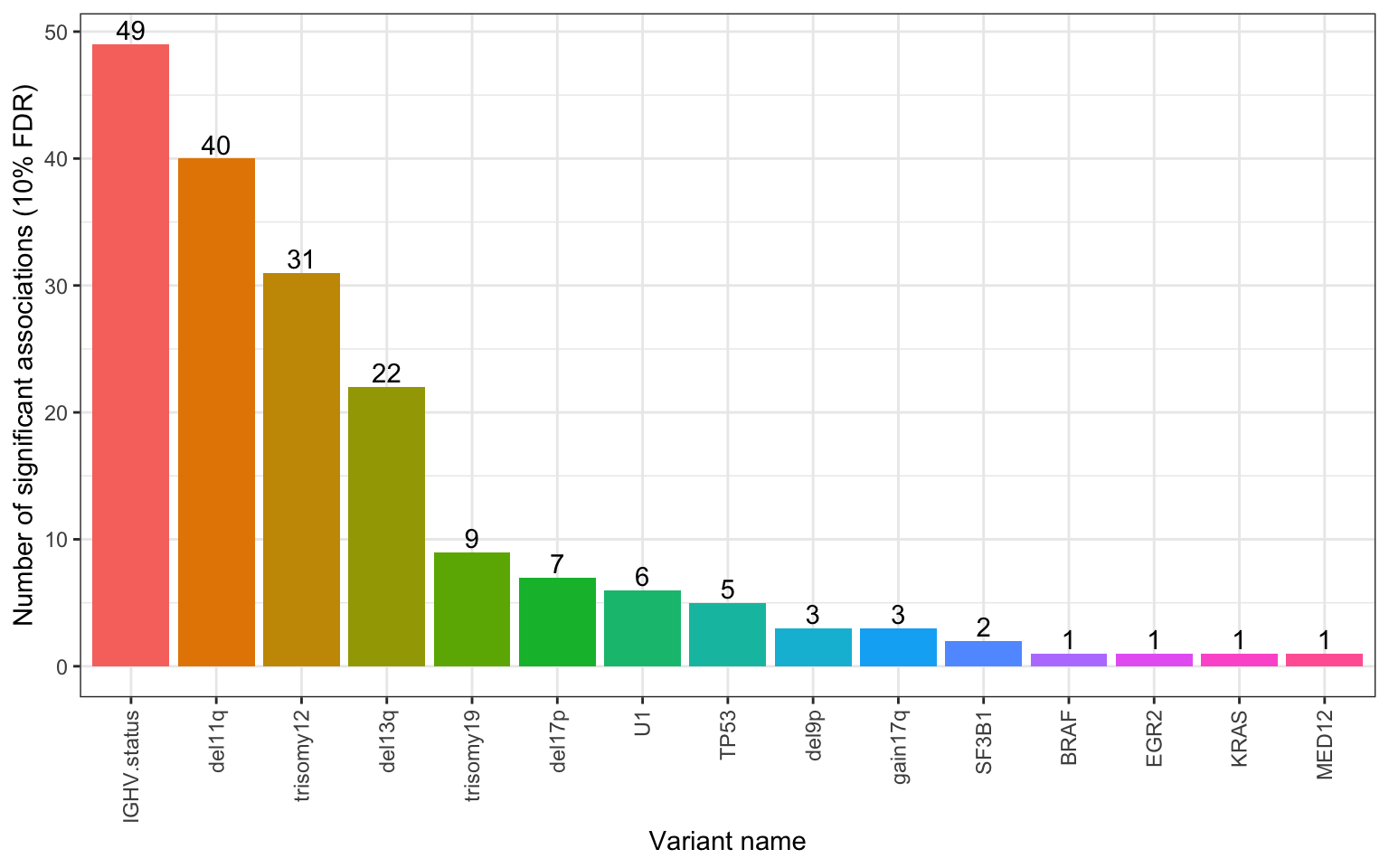
Number of significant associations per gene (10% FDR), adjusted by IHW
 Seems to help a little, especially with some each associations.
Use the result from p values adjustment by IHW
pTab <- mutate(pTab, p.adj = p.adj.ihw)P value scatter plot (only show drugs with assocations)
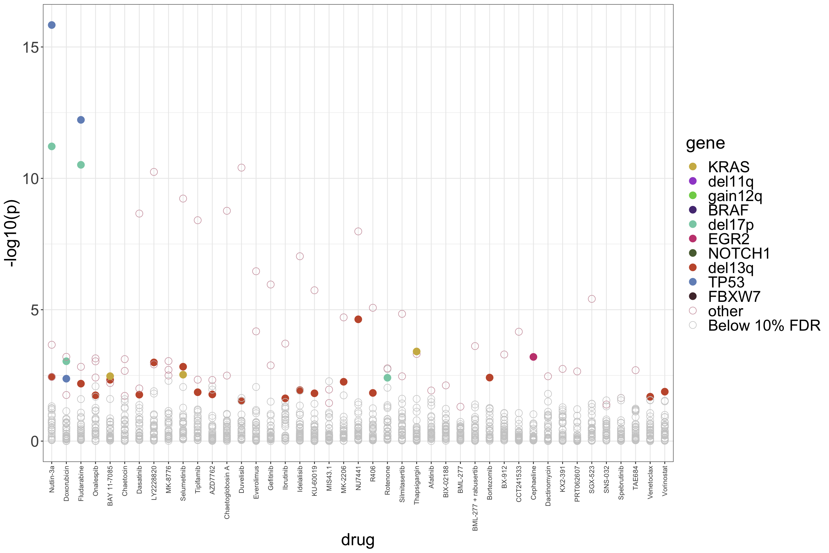
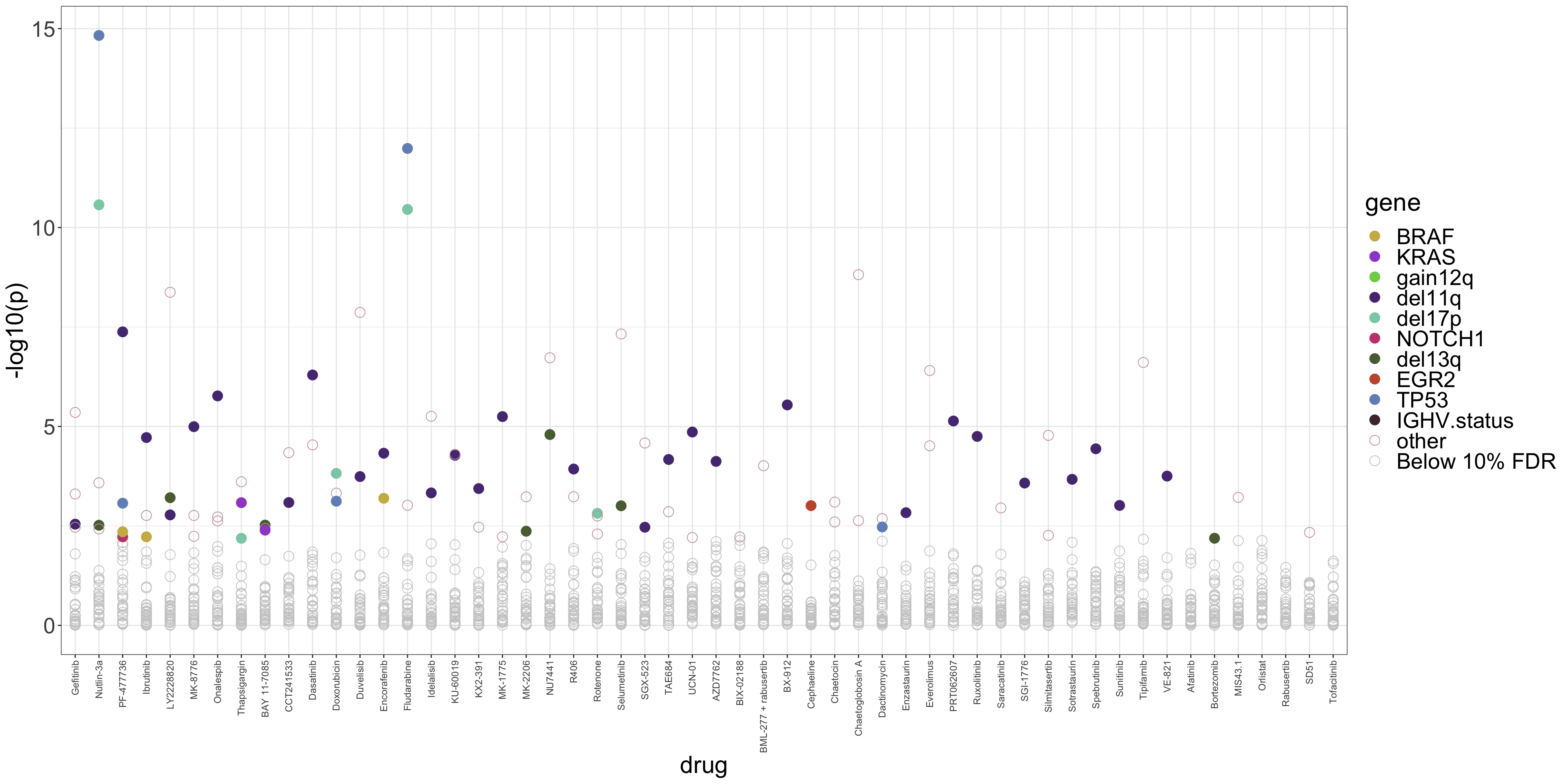 Associations pass 10% FDR are colored by genes.
Only a few associations pass the 10% FDR threshold, although many
associations pass raw p-value 0.01 threshold. This could be due to the
multiple hypothesis testing problem. We have more drugs in EMLB2016
screen than other screens. (I already pre-filtered the drugs that show
very little variance across samples.)
PDF version: pScatter-1.pdf
Volcano plots
#filter genes with significant assocaitions
useGene <- unique(filter(pTab, p.adj <=0.1)$gene)

#get top 10 most up and down regulated genes
upDrug <- lapply(unique(pTab$gene), function(n) {
  dplyr::filter(pTab, gene ==n, logFC >0) %>% top_n(10, -log10(p))
}) %>% bind_rows()

downDrug <- lapply(unique(pTab$gene), function(n) {
  dplyr::filter(pTab, gene == n, logFC  < 0) %>% top_n(10, -log10(p))
}) %>% bind_rows()

drugLab <- bind_rows(upDrug, downDrug) %>%
  filter(p.adj <0.1) %>%
  mutate(drugLabel = drug) %>% select(drug, gene, drugLabel)

plotList <- lapply(useGene, function(n) {
  eachTab <- filter(pTab, gene %in% n, !is.na(p)) %>%
    mutate(direction = ifelse(p.adj > 0.1, "n.s.",
                              ifelse(logFC>0, "resistant","sensitive"))) %>%
    left_join(drugLab, by = c("drug", "gene"))

  #pCut <- -log10(max(filter(eachTab, p.adj <=0.1)$p))
  pCut <- -log10(0.1)
  ggplot(eachTab, aes(x=logFC, y = -log10(p.adj))) +
    geom_point(aes(col = direction)) +
    ggrepel::geom_text_repel(aes(label = drugLabel), max.overlaps = 100) +
    scale_color_manual(values = c("n.s."="grey60","resistant" = "red","sensitive" = "blue")) +
    geom_hline(yintercept = pCut, linetype = "dashed", color = "orange") +
    ylab("-log10(adjusted P value)") + xlab("log2(fold change)") +
    ggtitle(sprintf("%s (mutated vs unmutated)", n)) +
    theme_bw() +
    theme(plot.title = element_text(hjust=0.5, size=15, face ="bold"),
          legend.position = "bottom",
          axis.text = element_text(size=14),
          axis.title = element_text(size=14))
})
plot_grid(plotlist = plotList, ncol=2)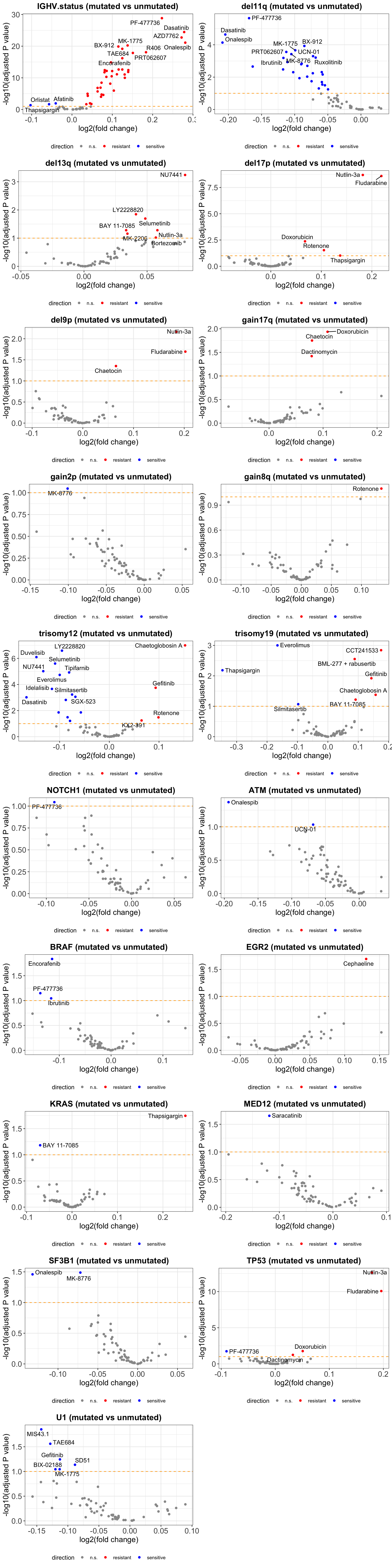
makepdf(plotList, "../docs/volcano_noBlocking_IC50.pdf", ncol=2, nrow=2, height = 10, width = 9)PDF version: volcano_noBlocking_IC50.pdf
A table of significant associations
filter(pTab, p.adj <=0.1) %>% mutate_if(is.numeric, formatC, digits=2) %>%
  DT::datatable()
Blocking for IGHV
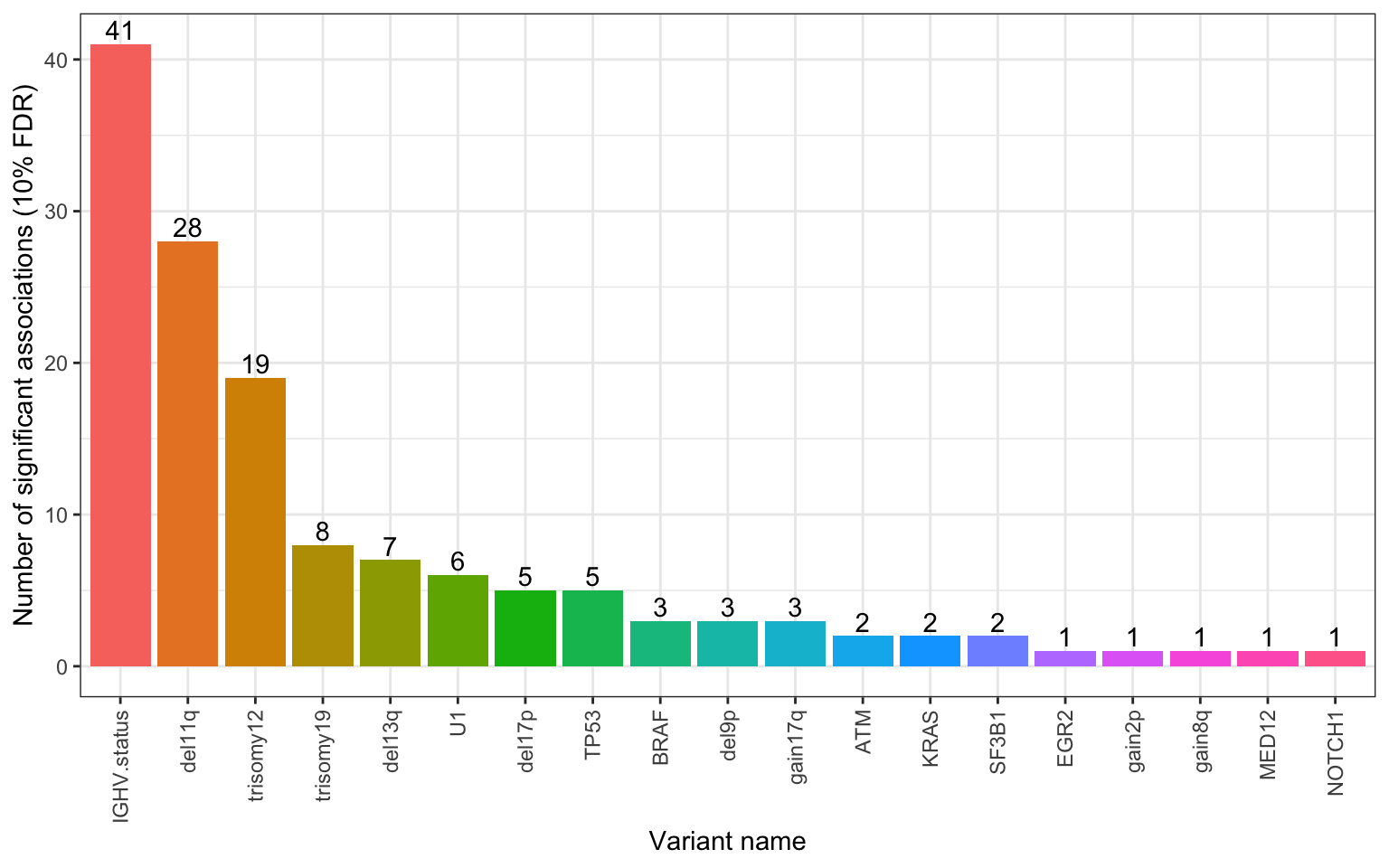
Number of significant associations per gene (10% FDR)
 Associations pass 10% FDR are colored by genes.
Number of significant associations per gene (10% FDR), adjusted by IHW
Number of significant associations per gene, blocking for non-IGHV features
P value scatter plot
 PDF version: pScatter_aov-1.pdf
Volcano plots
#filter genes with significant assocaitions
useGene <- unique(filter(pTab.block, p.adj <=0.1)$gene)

#get top 10 most up and down regulated genes
upDrug <- lapply(unique(pTab.block$gene), function(n) {
  filter(pTab.block, gene ==n, logFC >0) %>% top_n(10, -log10(p))
}) %>% bind_rows()

downDrug <- lapply(unique(pTab.block$gene), function(n) {
  filter(pTab.block, gene == n, logFC  < 0) %>% top_n(10, -log10(p))
}) %>% bind_rows()

drugLab <- bind_rows(upDrug, downDrug) %>%
  filter(p.adj <0.1) %>%
  mutate(drugLabel = drug) %>% select(drug, gene, drugLabel)

plotList <- lapply(useGene, function(n) {
  eachTab <- filter(pTab.block, gene %in% n, !is.na(p)) %>%
    mutate(direction = ifelse(p.adj > 0.1, "n.s.",
                              ifelse(logFC>0, "resistant","sensitive"))) %>%
    left_join(drugLab, by = c("drug", "gene"))

  #pCut <- -log10(max(filter(eachTab, p.adj <=0.1)$p))
  pCut <- -log10(0.1)
  ggplot(eachTab, aes(x=logFC, y = -log10(p.adj))) +
    geom_point(aes(col = direction)) +
    ggrepel::geom_text_repel(aes(label = drugLabel), max.overlaps = 100) +
    scale_color_manual(values = c("n.s."="grey60","resistant" = "red","sensitive" = "blue")) +
    geom_hline(yintercept = pCut, linetype = "dashed", color = "orange") +
    ylab("-log10(adjusted P value)") + xlab("log2(fold change)") +
    ggtitle(sprintf("%s (mutated vs unmutated)", n)) +
    theme_bw() +
    theme(plot.title = element_text(hjust=0.5, size=15, face ="bold"),
          legend.position = "bottom",
          axis.text = element_text(size=14),
          axis.title = element_text(size=14))
})
plot_grid(plotlist = plotList, ncol=2)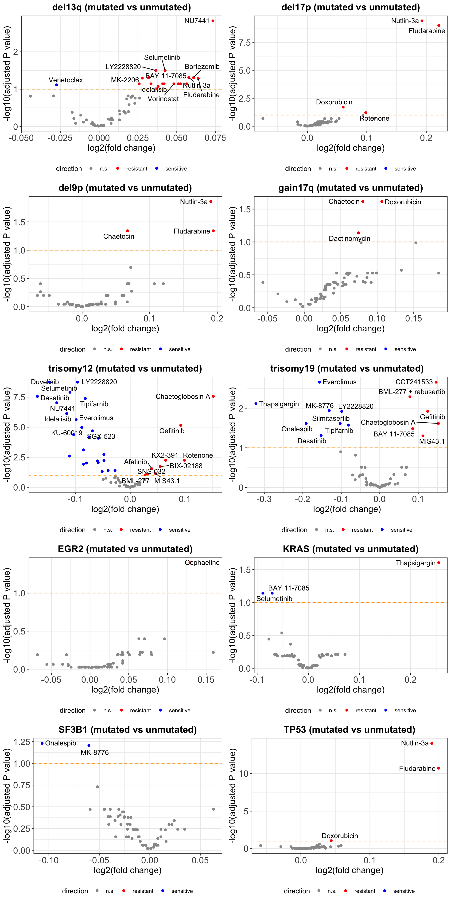
makepdf(plotList, "../docs/volcano_withBlocking_IC50.pdf", ncol=2, nrow=2, height = 10, width = 9)PDF version: volcano_withBlocking_IC50.pdf
A table of significant associations
filter(pTab.block, p.adj <=0.1) %>% mutate_if(is.numeric, formatC, digits=2) %>%
  DT::datatable()
Within M-CLL only
Only mutations occcured at least 3 times will be included in the test
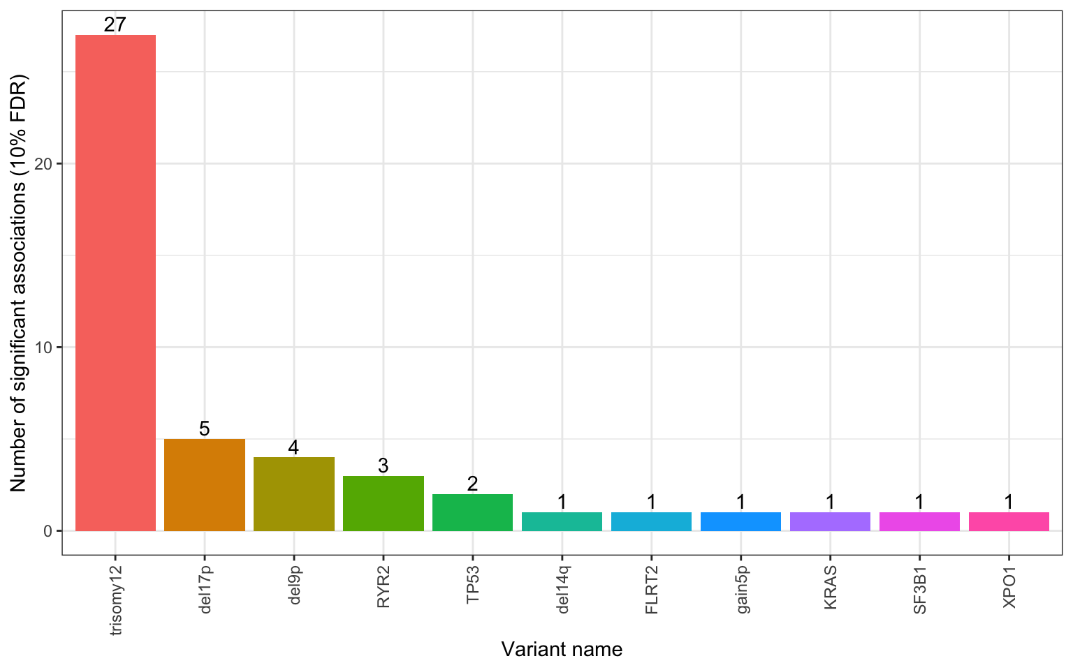
Number of significant associations per gene (10% FDR)
Volcano plots
#filter genes with significant assocaitions
useGene <- unique(filter(pTab, p.adj <=0.1)$gene)

plotList <- lapply(useGene, function(n) {
  eachTab <- filter(pTab, gene %in% n, !is.na(p)) %>%
    mutate(direction = ifelse(p.adj > 0.1, "n.s.",
                              ifelse(logFC>0, "resistant","sensitive"))) %>%
    mutate(drugLabel = ifelse(direction == "n.s.","",drug))

  pCut <- -log10(max(filter(eachTab, p.adj <=0.1)$p))

  ggplot(eachTab, aes(x=logFC, y = -log10(p))) +
    geom_point(aes(col = direction)) +
    ggrepel::geom_text_repel(aes(label = drugLabel), max.overlaps = 100) +
    scale_color_manual(values = c("n.s."="grey60","resistant" = "red","sensitive" = "blue")) +
    geom_hline(yintercept = pCut, linetype = "dashed", color = "orange") +
    ylab("-log10 (P value)") + xlab("log2 Fold Change") +
    ggtitle(sprintf("%s (mutated vs unmutated)", n)) +
    theme_bw() +
    theme(plot.title = element_text(hjust=0.5, size=15, face ="bold"),
          legend.position = "bottom")
})
plot_grid(plotlist = plotList, ncol=2)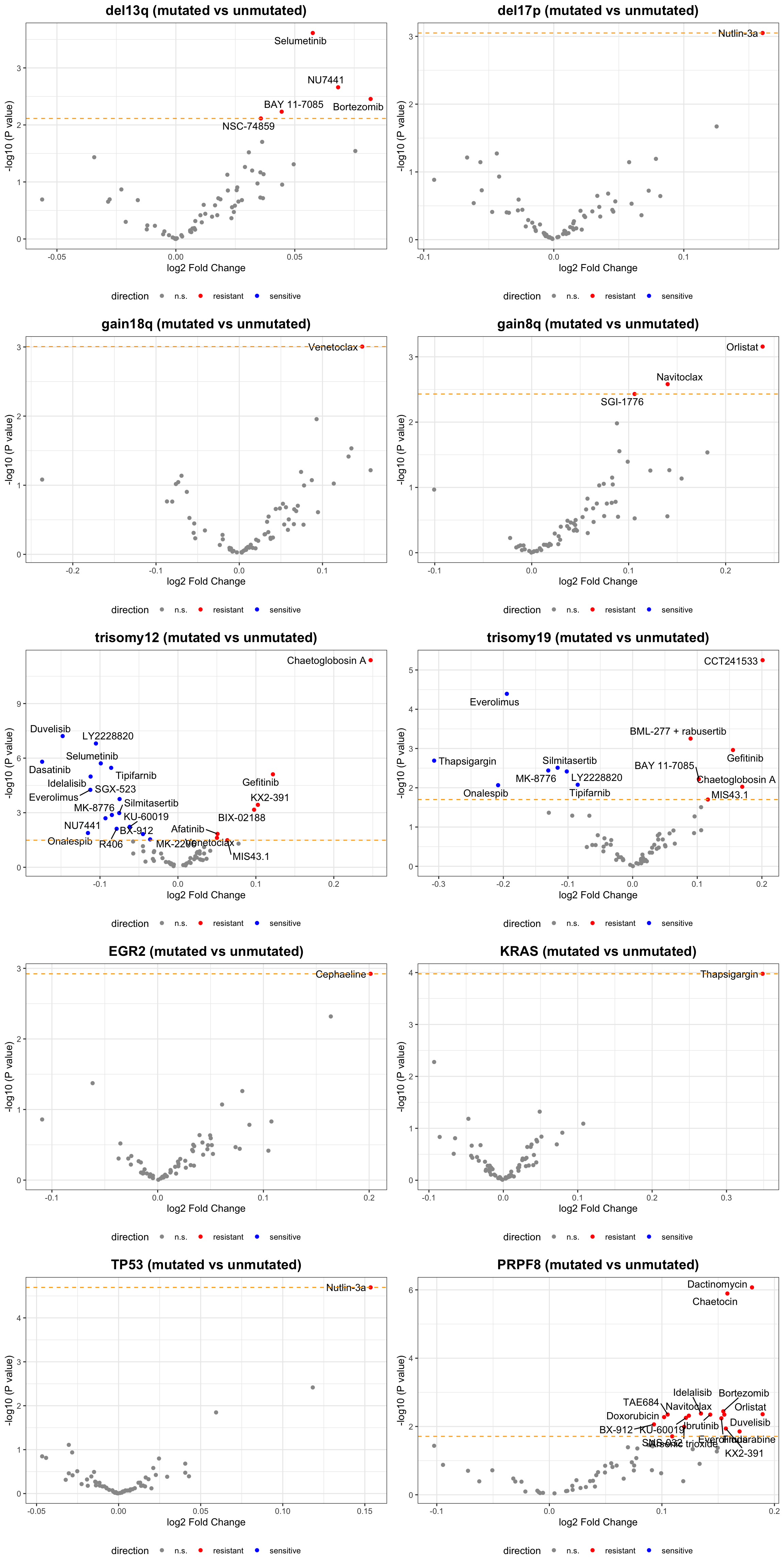
makepdf(plotList, "../docs/volcano_M_CLL_IC50.pdf", ncol=1, nrow=1, height = 12, width = 12)PDF version: volcano_M_CLL_IC50.pdf
A table of significant associations
filter(pTab, p.adj <=0.1) %>% mutate_if(is.numeric, formatC, digits=2) %>%
  DT::datatable()
Within U-CLL only
Only mutations occcured at least 3 times will be included in the test
Number of significant associations per gene (10% FDR)
Volcano plots
#filter genes with significant assocaitions
useGene <- unique(filter(pTab, p.adj <=0.1)$gene)

plotList <- lapply(useGene, function(n) {
  eachTab <- filter(pTab, gene %in% n, !is.na(p)) %>%
    mutate(direction = ifelse(p.adj > 0.1, "n.s.",
                              ifelse(logFC>0, "resistant","sensitive"))) %>%
    mutate(drugLabel = ifelse(direction == "n.s.","",drug))

  pCut <- -log10(max(filter(eachTab, p.adj <=0.1)$p))

  ggplot(eachTab, aes(x=logFC, y = -log10(p))) +
    geom_point(aes(col = direction)) +
    ggrepel::geom_text_repel(aes(label = drugLabel), max.overlaps = 100) +
    scale_color_manual(values = c("n.s."="grey60","resistant" = "red","sensitive" = "blue")) +
    geom_hline(yintercept = pCut, linetype = "dashed", color = "orange") +
    ylab("-log10 (P value)") + xlab("log2 Fold Change") +
    ggtitle(sprintf("%s (mutated vs unmutated)", n)) +
    theme_bw() +
    theme(plot.title = element_text(hjust=0.5, size=15, face ="bold"),
          legend.position = "bottom")
})
plot_grid(plotlist = plotList, ncol=2)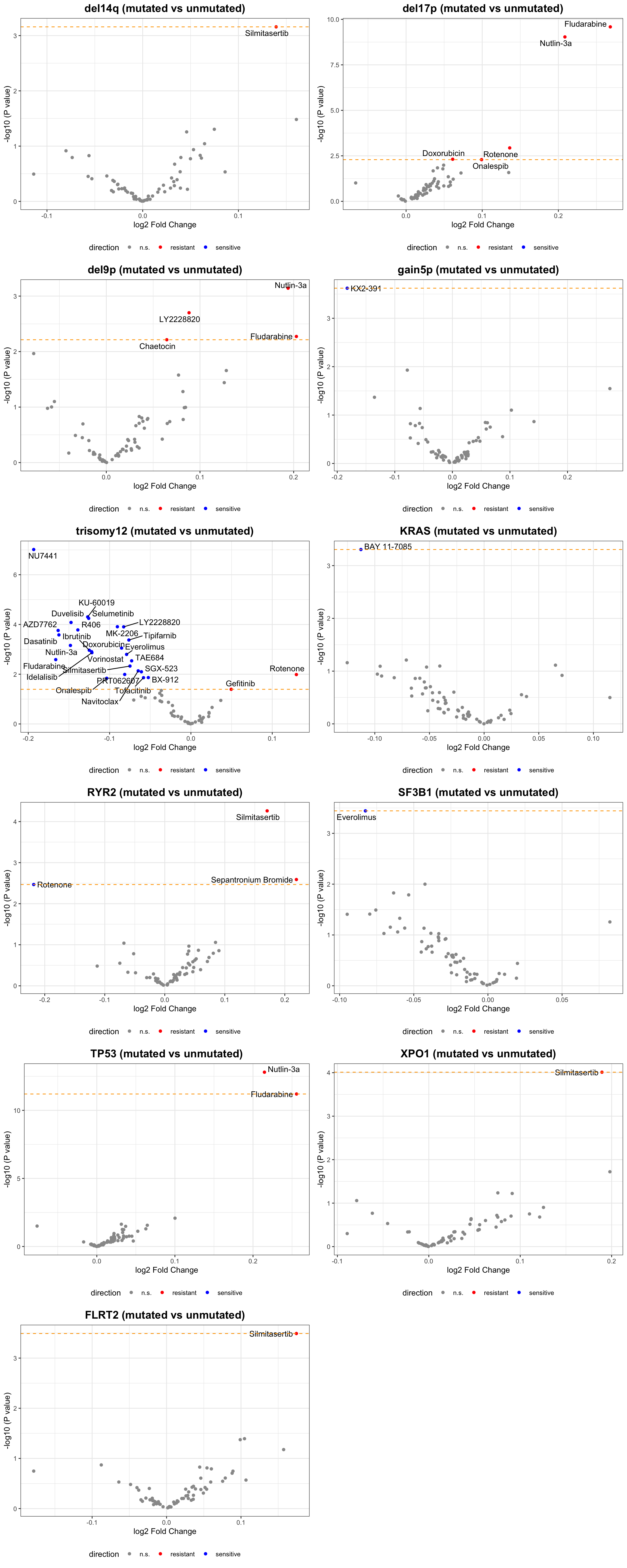
makepdf(plotList, "../docs/volcano_U_CLL_IC50.pdf", ncol=1, nrow=1, height = 12, width = 12)PDF version: volcano_U_CLL_IC50.pdf
A table of significant associations
filter(pTab, p.adj <=0.1) %>% mutate_if(is.numeric, formatC, digits=2) %>%
  DT::datatable()
Using individual concentrations
Without blocking for IGHV
p_table_noBlock_allConc_IC50.csv
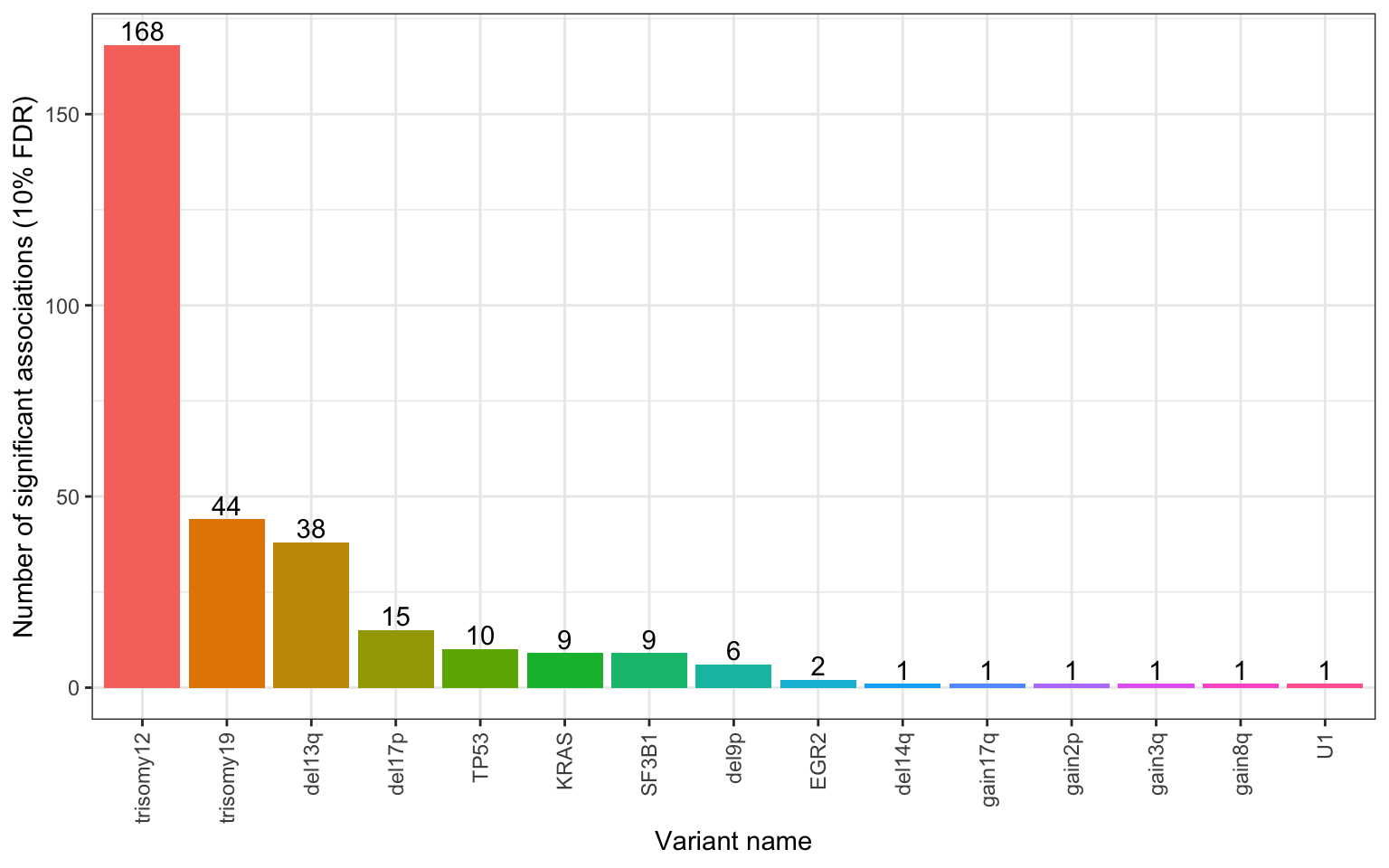
Number of significant associations per gene (10%
FDR)
P value heatmap
Only drugs show at least one significant association under 10% FDR
pTab.sig <- filter(pTab, p.adj <= 0.1)
plotTab <- filter(pTab, gene %in% pTab.sig$gene) %>%
filter(Drug %in% pTab.sig$Drug) %>%
mutate(sign = ifelse(p.adj <= 0.1, "*",""),
pSign = -log10(p)) %>%
mutate(pSign = ifelse(pSign > 12, 12, pSign)) %>%
mutate(pSign = pSign * sign(logFC),
Drug = sprintf("%s (%s)",Drug, targetFamily))
pMat <- mutate(plotTab, geneConc = paste0(gene,"_", concIndex)) %>%
select(Drug, geneConc, pSign) %>%
pivot_wider(names_from = geneConc, values_from = pSign) %>%
data.frame() %>% column_to_rownames("Drug")
hc <- hclust(dist(pMat))
drugOrder <- rownames(pMat)[hc$order]
plotTab <- mutate(plotTab, Drug = factor(Drug, levels = drugOrder),
gene = factor(gene, levels = levels(sumTab$gene)))
ggplot(plotTab, aes(x=concIndex, y = Drug, fill = pSign)) +
geom_tile() + geom_text(aes(label=sign), nudge_y = -0.25) +
scale_fill_gradient2(low = "blue", mid = "white", high = "red", name ="-log10(P-value)") +
facet_wrap(~gene, ncol =12) +
xlab("concentration index")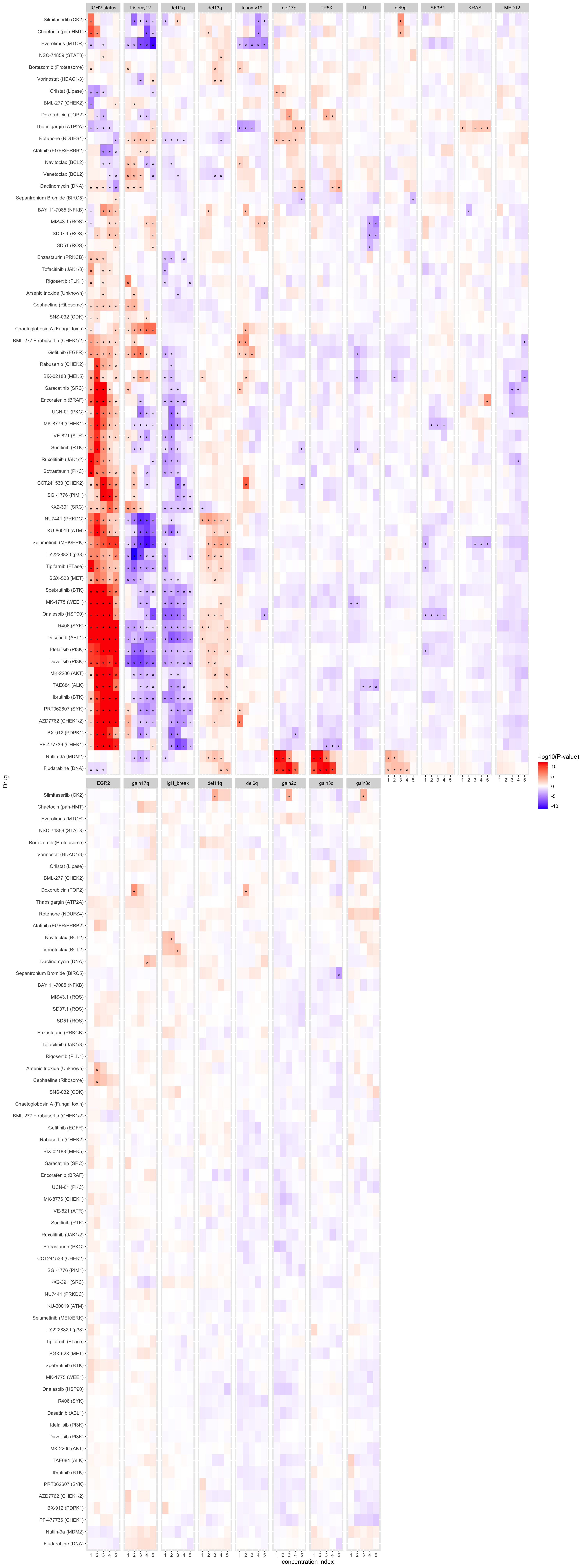 * indicates assocations passed 10% FDR control
A table of significant associations
filter(pTab, p.adj <=0.1) %>% mutate_if(is.numeric, formatC, digits=2) %>%
  left_join(select(targetAnno, drugName, target, pathway), by = c(Drug = "drugName")) %>%
  DT::datatable()
Blocking for IGHV
p_table_ighvBlock_allConc_IC50.csv
Number of significant associations per gene (10%
FDR)
P value heatmap
Only drugs show at least one significant association under 10% FDR
pTab.sig <- filter(pTab, p.adj <= 0.1)
plotTab <- filter(pTab, gene %in% pTab.sig$gene) %>%
filter(Drug %in% pTab.sig$Drug) %>%
mutate(sign = ifelse(p.adj <= 0.1, "*",""),
pSign = -log10(p)) %>%
mutate(pSign = ifelse(pSign > 12, 12, pSign)) %>%
mutate(pSign = pSign * sign(logFC),
Drug = sprintf("%s (%s)",Drug, targetFamily))
pMat <- mutate(plotTab, geneConc = paste0(gene,"_", concIndex)) %>%
select(Drug, geneConc, pSign) %>%
pivot_wider(names_from = geneConc, values_from = pSign) %>%
data.frame() %>% column_to_rownames("Drug")
hc <- hclust(dist(pMat))
drugOrder <- rownames(pMat)[hc$order]
plotTab <- mutate(plotTab, Drug = factor(Drug, levels = drugOrder),
gene = factor(gene, levels = levels(sumTab$gene)))
ggplot(plotTab, aes(x=concIndex, y = Drug, fill = pSign)) +
geom_tile() + geom_text(aes(label=sign), nudge_y = -0.25) +
scale_fill_gradient2(low = "blue", mid = "white", high = "red", name = "-log10(P-value)") +
facet_wrap(~gene, ncol =12) +
xlab("concentration index")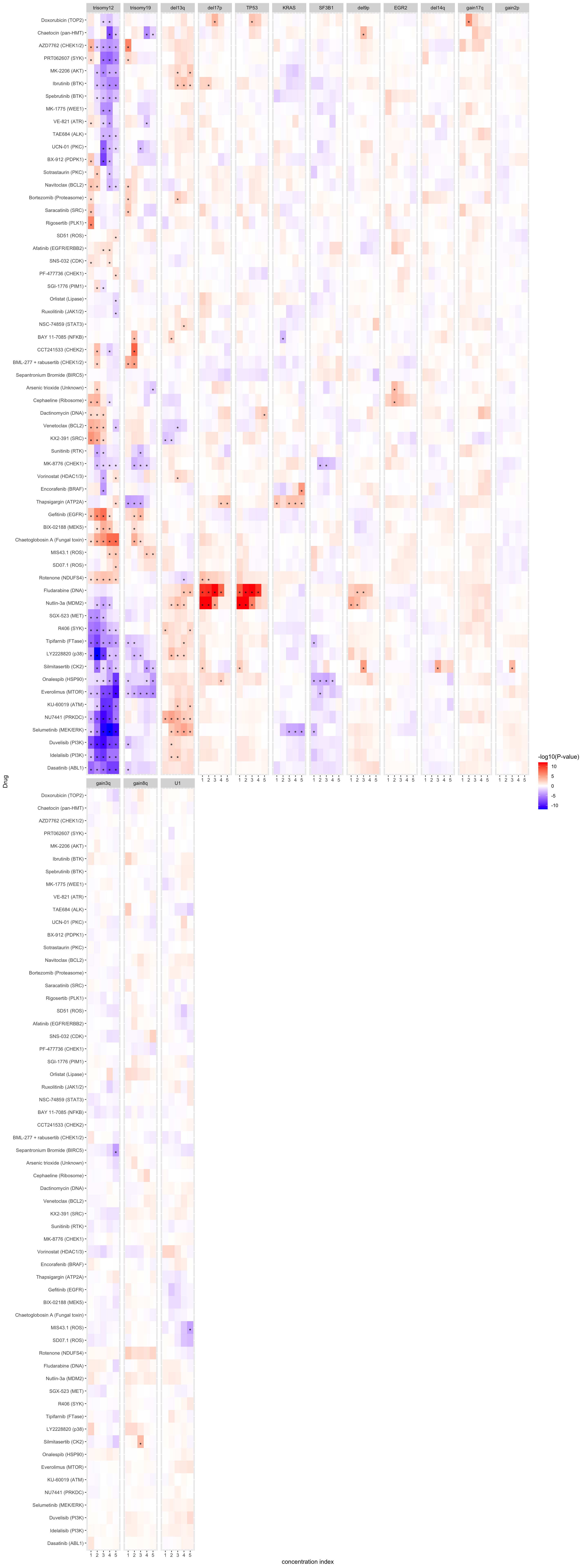 * indicates associations passed 10% FDR control
A table of significant associations
targetAnno <- read_csv2("../data/targetAnnotation_all.csv") %>%
  mutate(drugName = nameEMBL2016)

filter(pTab, p.adj <=0.1) %>% mutate_if(is.numeric, formatC, digits=2) %>%
  left_join(select(targetAnno, drugName, target, pathway), by = c(Drug = "drugName")) %>%
  DT::datatable()
Drug responses associated with IGHV
Volcano plot
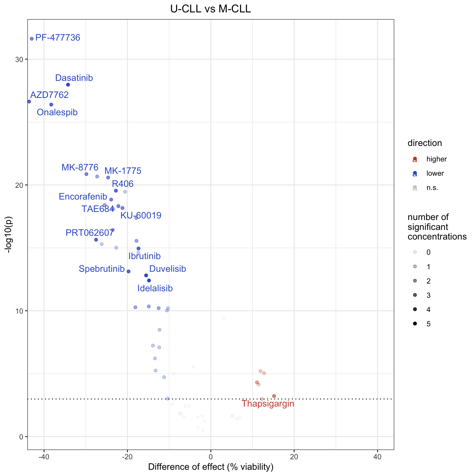 Drugs colored by blue are more effective in U-CLL samples. The names of
the drugs that show significant associations and effect size above 10%
in at least 3 concentrations are labeled. Dashed line indicates 5%
FDR
Drugs colored by blue are more effective in U-CLL samples. The names of
the drugs that show significant associations and effect size above 10%
in at least 3 concentrations are labeled. Dashed line indicates 5%
FDR
As expected, M-CLL samples show increased resistance to a lot of drugs.
Drug responses associated with Trisomy12
For all CLLs
How many triosmy12 samples?
tri12Tab <- distinct(viabTab, patientID, .keep_all = TRUE)
tri12Tab %>% filter(trisomy12 == 1) %>% nrow()
[1] 27Volcano plot (10% FDR cut-off) for combined
concentrations
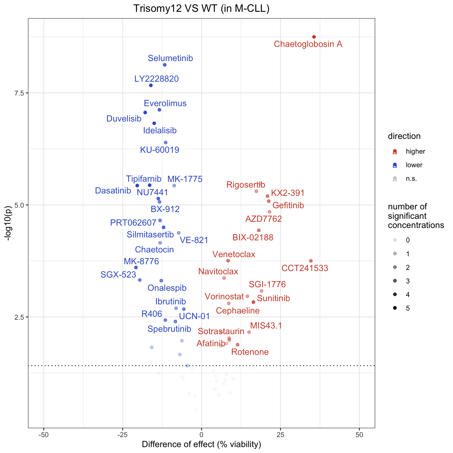
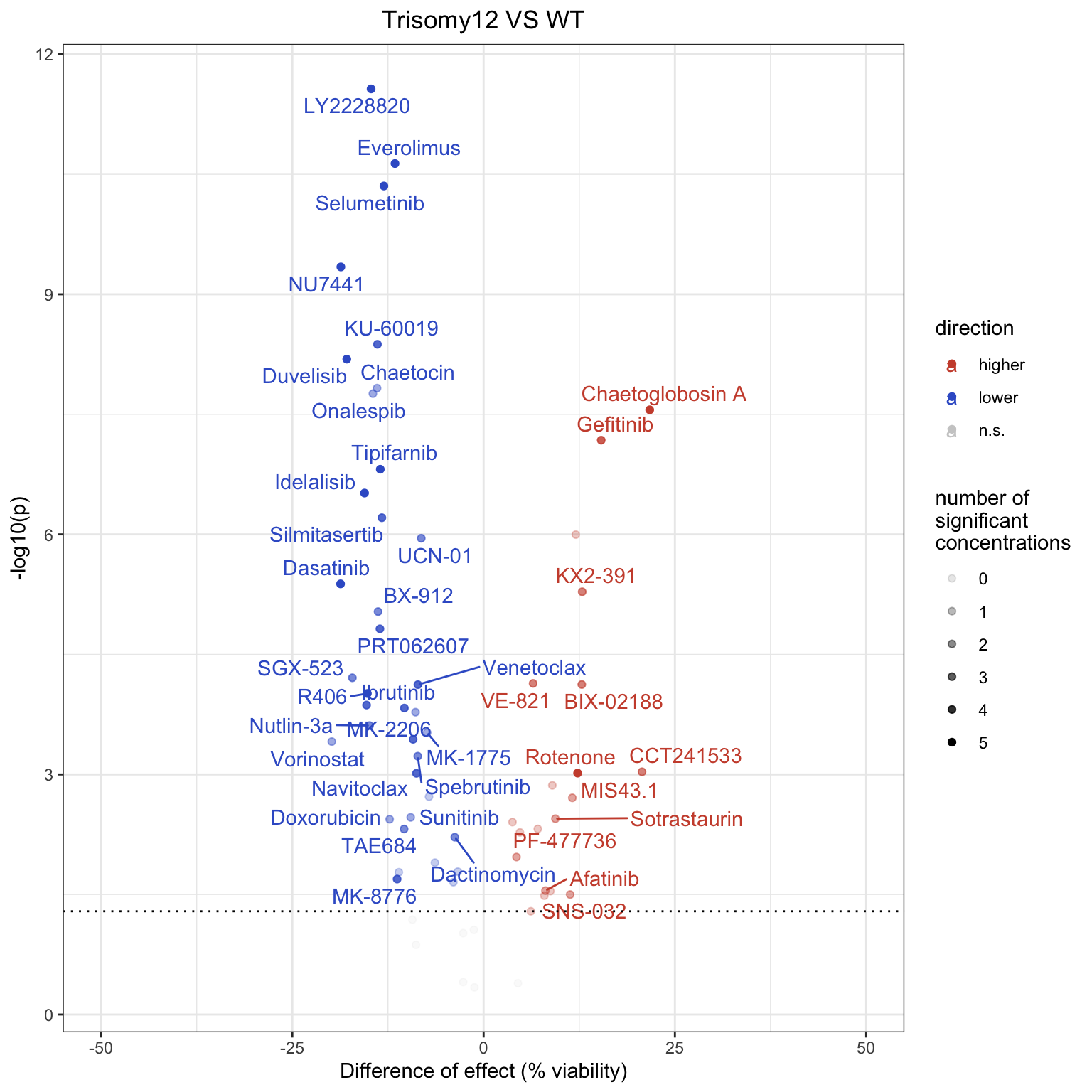 Drugs colored by blue are more effective in samples with trisomy12. The
names of the drugs that show significant associations in at least 2
concentrations are labeled. Dashed line indicates 10% FDR.
Drugs colored by blue are more effective in samples with trisomy12. The
names of the drugs that show significant associations in at least 2
concentrations are labeled. Dashed line indicates 10% FDR.
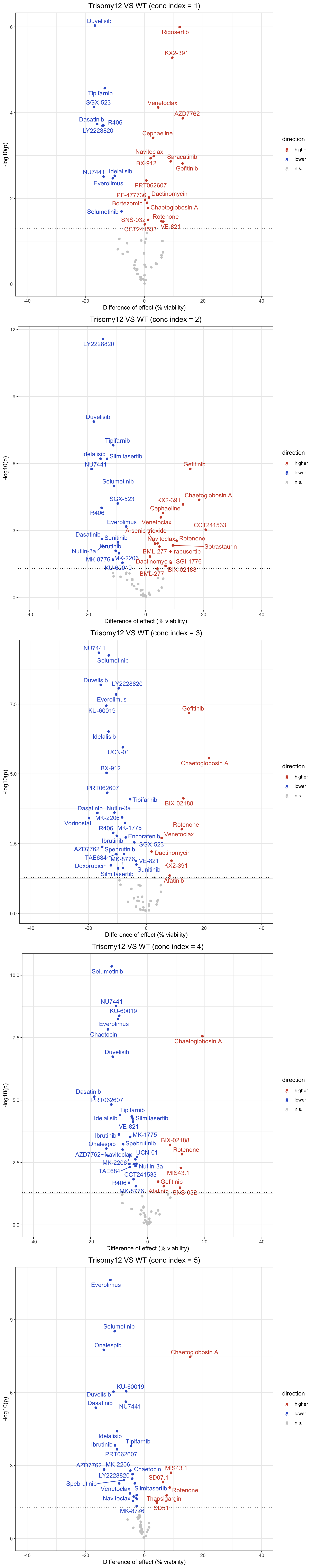
Volcano plots for individual concentrations
Beeswarm plots for all drug at all concentrations
For M CLLs only
Volcano plot (combined concentrations)
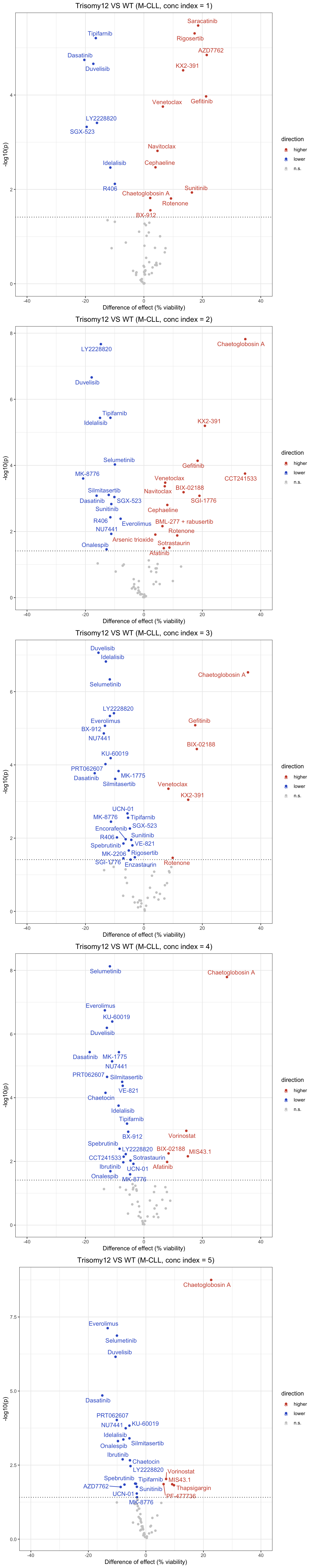
Volcation plots for individual concentrations
Beeswarm plots for all drug at all concentrations
For U CLLs
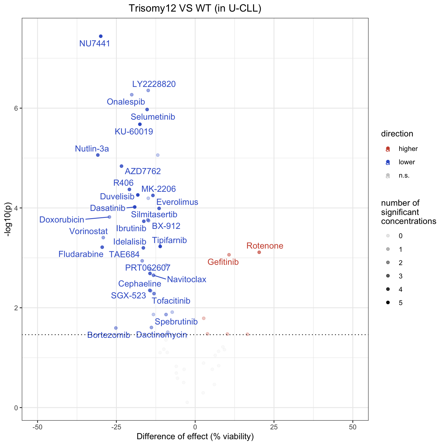
Volcano plot (combined concentrations)
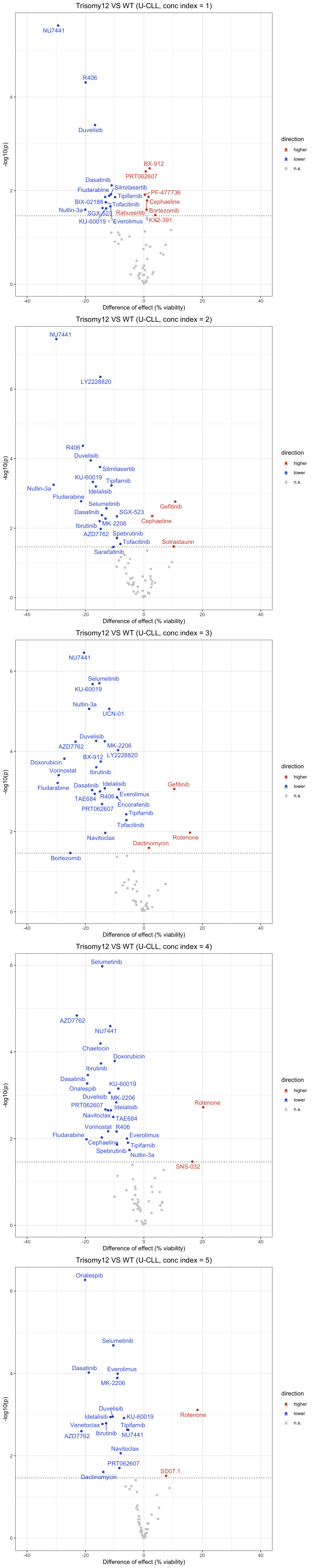
Volcation plots for individual concentrations
Beeswarm plots for all drug at all concentrations
Drug_VS_trisomy12_allConc_U-CLL_IC50.pdf
sessionInfo()R version 4.2.0 (2022-04-22)
Platform: x86_64-apple-darwin17.0 (64-bit)
Running under: macOS Big Sur/Monterey 10.16
Matrix products: default
BLAS: /Library/Frameworks/R.framework/Versions/4.2/Resources/lib/libRblas.0.dylib
LAPACK: /Library/Frameworks/R.framework/Versions/4.2/Resources/lib/libRlapack.dylib
locale:
[1] en_US.UTF-8/en_US.UTF-8/en_US.UTF-8/C/en_US.UTF-8/en_US.UTF-8
attached base packages:
[1] stats graphics grDevices utils datasets methods base
other attached packages:
[1] forcats_0.5.1 stringr_1.4.0 dplyr_1.0.9
[4] purrr_0.3.4 readr_2.1.2 tidyr_1.2.0
[7] tibble_3.1.7 tidyverse_1.3.1 limma_3.52.1
[10] IHW_1.24.0 readxl_1.4.0 gtable_0.3.0
[13] ggbeeswarm_0.6.0 jyluMisc_0.1.5 colorspace_2.0-3
[16] RColorBrewer_1.1-3 ggrepel_0.9.1 ggplot2_3.3.6
[19] cowplot_1.1.1 genefilter_1.78.0 pheatmap_1.0.12
[22] reshape2_1.4.4 gridExtra_2.3 Biobase_2.56.0
[25] BiocGenerics_0.42.0
loaded via a namespace (and not attached):
[1] utf8_1.2.2 shinydashboard_0.7.2
[3] tidyselect_1.1.2 RSQLite_2.2.14
[5] AnnotationDbi_1.58.0 htmlwidgets_1.5.4
[7] grid_4.2.0 BiocParallel_1.30.2
[9] maxstat_0.7-25 munsell_0.5.0
[11] codetools_0.2-18 DT_0.23
[13] withr_2.5.0 highr_0.9
[15] knitr_1.39 rstudioapi_0.13
[17] stats4_4.2.0 ggsignif_0.6.3
[19] MatrixGenerics_1.8.0 labeling_0.4.2
[21] git2r_0.30.1 slam_0.1-50
[23] GenomeInfoDbData_1.2.8 lpsymphony_1.24.0
[25] KMsurv_0.1-5 bit64_4.0.5
[27] farver_2.1.0 rprojroot_2.0.3
[29] vctrs_0.4.1 generics_0.1.2
[31] TH.data_1.1-1 xfun_0.31
[33] sets_1.0-21 R6_2.5.1
[35] GenomeInfoDb_1.32.2 bitops_1.0-7
[37] cachem_1.0.6 fgsea_1.22.0
[39] DelayedArray_0.22.0 assertthat_0.2.1
[41] promises_1.2.0.1 scales_1.2.0
[43] vroom_1.5.7 multcomp_1.4-19
[45] beeswarm_0.4.0 sandwich_3.0-1
[47] workflowr_1.7.0 rlang_1.0.2
[49] splines_4.2.0 rstatix_0.7.0
[51] broom_0.8.0 BiocManager_1.30.18
[53] yaml_2.3.5 abind_1.4-5
[55] modelr_0.1.8 crosstalk_1.2.0
[57] backports_1.4.1 httpuv_1.6.5
[59] tools_4.2.0 relations_0.6-12
[61] ellipsis_0.3.2 gplots_3.1.3
[63] jquerylib_0.1.4 Rcpp_1.0.8.3
[65] plyr_1.8.7 visNetwork_2.1.0
[67] zlibbioc_1.42.0 RCurl_1.98-1.6
[69] ggpubr_0.4.0 S4Vectors_0.34.0
[71] zoo_1.8-10 SummarizedExperiment_1.26.1
[73] haven_2.5.0 cluster_2.1.3
[75] exactRankTests_0.8-35 fs_1.5.2
[77] magrittr_2.0.3 data.table_1.14.2
[79] reprex_2.0.1 survminer_0.4.9
[81] mvtnorm_1.1-3 matrixStats_0.62.0
[83] hms_1.1.1 shinyjs_2.1.0
[85] mime_0.12 evaluate_0.15
[87] xtable_1.8-4 XML_3.99-0.9
[89] IRanges_2.30.0 compiler_4.2.0
[91] KernSmooth_2.23-20 crayon_1.5.1
[93] htmltools_0.5.2 later_1.3.0
[95] tzdb_0.3.0 lubridate_1.8.0
[97] DBI_1.1.2 dbplyr_2.1.1
[99] MASS_7.3-57 BiocStyle_2.24.0
[101] Matrix_1.4-1 car_3.0-13
[103] cli_3.3.0 marray_1.74.0
[105] parallel_4.2.0 igraph_1.3.1
[107] GenomicRanges_1.48.0 pkgconfig_2.0.3
[109] km.ci_0.5-6 piano_2.12.0
[111] xml2_1.3.3 annotate_1.74.0
[113] vipor_0.4.5 bslib_0.3.1
[115] XVector_0.36.0 drc_3.0-1
[117] rvest_1.0.2 digest_0.6.29
[119] Biostrings_2.64.0 rmarkdown_2.14
[121] cellranger_1.1.0 fastmatch_1.1-3
[123] survMisc_0.5.6 shiny_1.7.1
[125] gtools_3.9.2 lifecycle_1.0.1
[127] jsonlite_1.8.0 carData_3.0-5
[129] fansi_1.0.3 pillar_1.7.0
[131] lattice_0.20-45 KEGGREST_1.36.0
[133] fastmap_1.1.0 httr_1.4.3
[135] plotrix_3.8-2 survival_3.3-1
[137] glue_1.6.2 fdrtool_1.2.17
[139] png_0.1-7 bit_4.0.4
[141] stringi_1.7.6 sass_0.4.1
[143] blob_1.2.3 caTools_1.18.2
[145] memoise_2.0.1