Overview of cohort composition and drug response pattern
Junyan Lu
4 November 2022
Last updated: 2022-11-04
Checks: 6 1
Knit directory: EMBL2016/analysis/
This reproducible R Markdown analysis was created with workflowr (version 1.7.0). The Checks tab describes the reproducibility checks that were applied when the results were created. The Past versions tab lists the development history.
The R Markdown is untracked by Git. To know which version of the R
Markdown file created these results, you’ll want to first commit it to
the Git repo. If you’re still working on the analysis, you can ignore
this warning. When you’re finished, you can run
wflow_publish to commit the R Markdown file and build the
HTML.
Great job! The global environment was empty. Objects defined in the global environment can affect the analysis in your R Markdown file in unknown ways. For reproduciblity it’s best to always run the code in an empty environment.
The command set.seed(20210512) was run prior to running
the code in the R Markdown file. Setting a seed ensures that any results
that rely on randomness, e.g. subsampling or permutations, are
reproducible.
Great job! Recording the operating system, R version, and package versions is critical for reproducibility.
Nice! There were no cached chunks for this analysis, so you can be confident that you successfully produced the results during this run.
Great job! Using relative paths to the files within your workflowr project makes it easier to run your code on other machines.
Great! You are using Git for version control. Tracking code development and connecting the code version to the results is critical for reproducibility.
The results in this page were generated with repository version 12d1722. See the Past versions tab to see a history of the changes made to the R Markdown and HTML files.
Note that you need to be careful to ensure that all relevant files for
the analysis have been committed to Git prior to generating the results
(you can use wflow_publish or
wflow_git_commit). workflowr only checks the R Markdown
file, but you know if there are other scripts or data files that it
depends on. Below is the status of the Git repository when the results
were generated:
Ignored files:
    Ignored:    .DS_Store
    Ignored:    .Rhistory
    Ignored:    .Rproj.user/
    Ignored:    analysis/.DS_Store
    Ignored:    analysis/.RData
    Ignored:    analysis/.Rhistory
    Ignored:    analysis/CDK_analysis_cache/
    Ignored:    analysis/boxplot_AUC.png
    Ignored:    analysis/consensus_clustering_CPS_cache/
    Ignored:    analysis/consensus_clustering_noFit_cache/
    Ignored:    analysis/dose_curve.png
    Ignored:    analysis/targetDist.png
    Ignored:    analysis/toxivity_box.png
    Ignored:    analysis/volcano.png
    Ignored:    data/.DS_Store
    Ignored:    output/.DS_Store

Untracked files:
    Untracked:  analysis/AUC_CLL_IC50/
    Untracked:  analysis/BRAF_analysis.Rmd
    Untracked:  analysis/CDK_analysis.Rmd
    Untracked:  analysis/GSVA_analysis.Rmd
    Untracked:  analysis/MOFA_analysis.Rmd
    Untracked:  analysis/NOTCH1_signature.Rmd
    Untracked:  analysis/autoluminescence.Rmd
    Untracked:  analysis/bar_plot_mixed_noU1.pdf
    Untracked:  analysis/beatAML/
    Untracked:  analysis/consensus_clustering.Rmd
    Untracked:  analysis/consensus_clustering_CPS.Rmd
    Untracked:  analysis/consensus_clustering_IC50.Rmd
    Untracked:  analysis/consensus_clustering_beatAML.Rmd
    Untracked:  analysis/consensus_clustering_noFit.Rmd
    Untracked:  analysis/coxResTab.RData
    Untracked:  analysis/disease_specific.Rmd
    Untracked:  analysis/drugScreens_reproducibility.Rmd
    Untracked:  analysis/genomic_association.Rmd
    Untracked:  analysis/genomic_association_IC50.Rmd
    Untracked:  analysis/genomic_association_allDisease.Rmd
    Untracked:  analysis/noFit_CLL/
    Untracked:  analysis/outcome_associations.Rmd
    Untracked:  analysis/overview.Rmd
    Untracked:  analysis/plotCohort.Rmd
    Untracked:  analysis/preprocess.Rmd
    Untracked:  code/utils.R
    Untracked:  data/BeatAML_Waves1_2/
    Untracked:  data/ic50Tab.RData
    Untracked:  data/newEMBL_20210806.RData
    Untracked:  data/patMeta.RData
    Untracked:  data/targetAnnotation_all.csv
    Untracked:  output/gene_associations/
    Untracked:  output/mofaRes.rds
    Untracked:  output/resConsClust.RData
    Untracked:  output/resConsClust_aucFit.RData
    Untracked:  output/resConsClust_beatAML.RData
    Untracked:  output/resConsClust_cps.RData
    Untracked:  output/resConsClust_ic50.RData
    Untracked:  output/resConsClust_noFit.RData
    Untracked:  output/screenData.RData

Unstaged changes:
    Modified:   _workflowr.yml
    Modified:   analysis/_site.yml
    Deleted:    analysis/about.Rmd
    Modified:   analysis/index.Rmd
    Deleted:    analysis/license.Rmd
Note that any generated files, e.g. HTML, png, CSS, etc., are not included in this status report because it is ok for generated content to have uncommitted changes.
There are no past versions. Publish this analysis with
wflow_publish() to start tracking its development.
Load libraries and dataset
#Libraries
library(Biobase)
library(gridExtra)
library(reshape2)
library(pheatmap)
library(genefilter)
library(cowplot)
library(Rtsne)
library(smallvis)
library(ggrepel)
library(RColorBrewer)
library(colorspace)
library(jyluMisc)
library(ggplot2)
library(ggbeeswarm)
library(gtable)
library(readxl)
library(limma)
library(tidyverse)

knitr::opts_chunk$set(message = FALSE, warning = FALSE, message = FALSE)
Load datasets
load("../data/patMeta.RData")
load("../output/screenData.RData")
Characterization of patients and drugs
Characterization of drugs
plotTab <- distinct(screenData, Drug, class) %>%
  group_by(class) %>% summarise(value = length(Drug)) %>%
  arrange(desc(value)) %>%
  mutate(text_y = cumsum(value) - value/2) %>%
  mutate(class = as.character(class))

df2 <- distinct(screenData, Drug, class) %>%
  group_by(class) %>% summarise(value = length(Drug)) %>%
  mutate(csum = rev(cumsum(rev(value))),
         pos = value/2 + lead(csum, 1),
         pos = if_else(is.na(pos), value/2, pos))

ggplot(df2, aes(x = "" , y = value, fill = fct_inorder(class))) +
  geom_col(width = 1, color = 1) +
  coord_polar(theta = "y") +
  geom_label_repel(data = df2,
                   aes(y = pos, label = class), fill = "grey80",
                   size = 6, nudge_x = 0.5, show.legend = FALSE) +
  theme_void() +
theme(legend.position = "none") 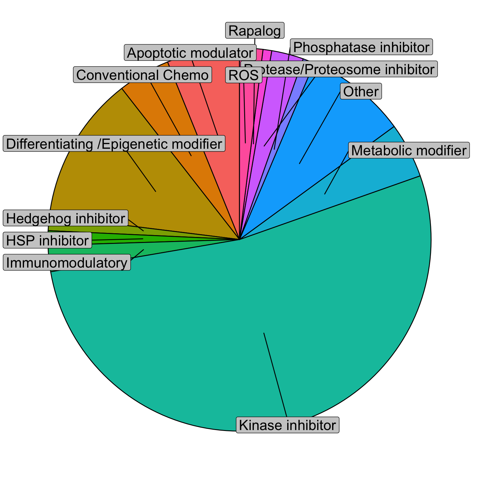
Target distribution of kinase inhibitors
tarAnno <- read_csv2("~/CLLproject_jlu/data/targetAnno/targetAnnotation_all.csv")
plotTab <- distinct(screenData, Drug, class) %>% mutate(target = tarAnno[match(Drug, tarAnno$nameEMBL2016),]$pathway) %>%
  filter(class == "Kinase inhibitor", !is.na(target)) %>%
  group_by(target) %>% summarise(n=length(Drug)) %>%
  arrange(desc(n)) %>% mutate(target = factor(target, levels = target))

ggplot(plotTab, aes(x=target, y=n)) +
  geom_bar(stat="identity", fill = "lightblue") +
  ylab("Number of drugs") + xlab("") +
  theme_bw() +
theme(axis.text.x = element_text(angle = 90, hjust=1, vjust=0.5)) 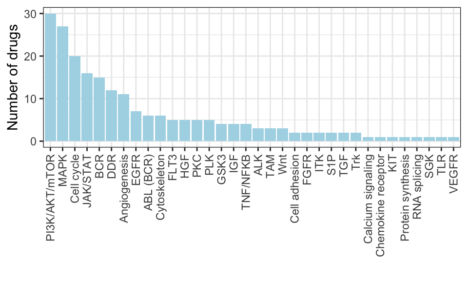
ggsave("targetDist.png", height = 3, width = 5)Summary of diagnosis
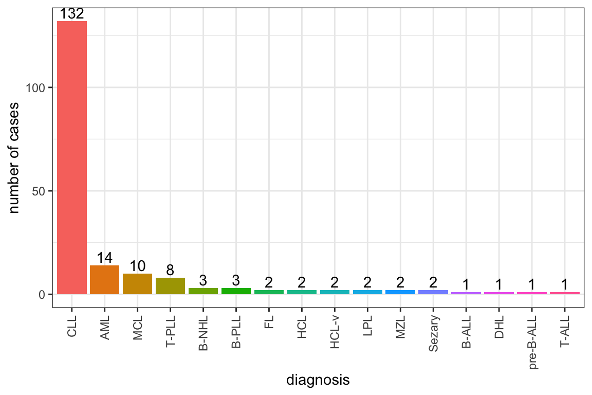
Summary of patient background
#Get a patient background table for EBML2016 patients
patBack <- filter(patMeta, Patient.ID %in% screenData$patientID) %>%
  mutate(sampleID = screenData[match(Patient.ID, screenData$patientID),]$sampleID) %>%
  mutate(pretreat = treatmentTab[match(sampleID, treatmentTab$sampleID),]$pretreat) %>% #add pretreatment status
  select(-project, -date.of.diagnosis, -treatment, -date.of.first.treatment, -HIPO.ID) %>%
  dplyr::rename(sex = gender)
Mutation statistics (for all patients)
# Get a mutation matrix and remove non-important features (CNV, SNV)
mutTab <- select(patBack, -sex, -diagnosis, -Methylation_Cluster, -pretreat) %>%
  mutate(IGHV.status = ifelse(is.na(IGHV.status), NA, ifelse(IGHV.status == "M",1,0))) %>%
  mutate_at(vars(-Patient.ID), as.character) %>% mutate_at(vars(-Patient.ID), as.integer) %>%
  data.frame() %>% remove_rownames() %>% column_to_rownames("Patient.ID")

#only keep the features that have at least 10 records with 5 positive/negative cases
keepCols <- apply(mutTab, 2, function(x) length(table(x)) >=2 & all(table(x) >=5))
mutTab <- mutTab[,keepCols]

#summary mutated, unmutated and NA cases
mutStat <- rownames_to_column(mutTab, "patID") %>% gather(key = "variant", value = "status", -patID) %>%
  mutate(status = ifelse(is.na(status), "unkown", ifelse(status == 0, "wt","mut"))) %>%
  mutate(status = factor(status, levels = c("mut","wt","unkown"))) %>%
  group_by(variant, status) %>% summarise(count = length(status)) %>% ungroup()

#reorder the variant by number of mutated cases
mutStat <- mutate(mutStat,
                  variant = factor(variant, levels = filter(mutStat, status == "mut") %>%
                                     arrange(count) %>% pull(variant)))

ggplot(mutStat, aes(x = variant, y = count, fill = status)) +
  geom_bar(stat = "identity", position = "dodge") +
  scale_fill_manual(values = c(mut = "pink", wt = "lightblue", unkown = "grey60")) +
  geom_text(aes(label=count), position=position_dodge(width=0.9), hjust=-0.25) +
  theme_classic()  +
  ylab("number of cases") + xlab("") + coord_flip()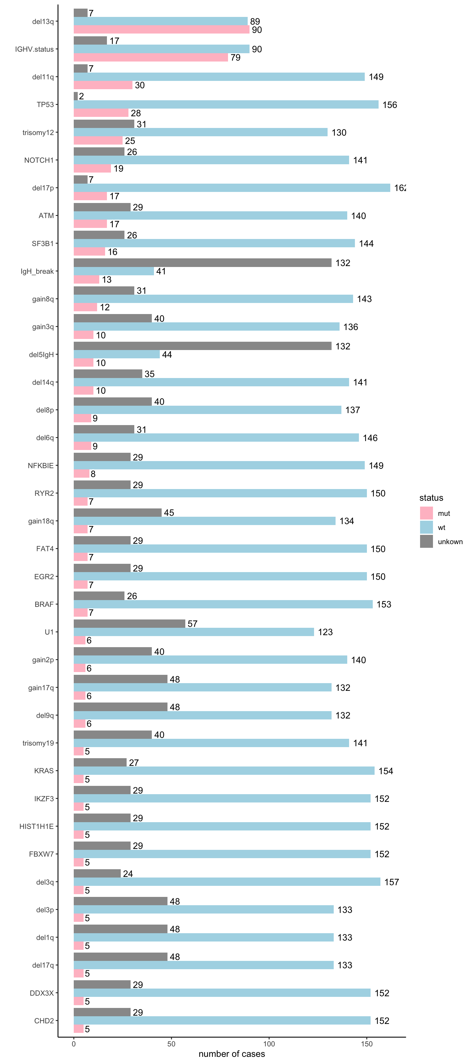
Mutation statistics (only for CLL patients)
# Get a mutation matrix and remove non-important features (CNV, SNV)
mutTab <- filter(patBack, diagnosis %in% "CLL") %>%
  select(-sex, -diagnosis, -Methylation_Cluster, -pretreat) %>%
  mutate(IGHV.status = ifelse(is.na(IGHV.status), NA, ifelse(IGHV.status == "M",1,0))) %>%
  mutate_at(vars(-Patient.ID), as.character) %>% mutate_at(vars(-Patient.ID), as.integer) %>%
  data.frame() %>% remove_rownames() %>% column_to_rownames("Patient.ID")

#only keep the features that have at least 10 records with 5 positive/negative cases
keepCols <- apply(mutTab, 2, function(x) length(table(x))>=2 & all(table(x) >=5))
mutTab <- mutTab[,keepCols]

#summary mutated, unmutated and NA cases
mutStat <- rownames_to_column(mutTab, "patID") %>% gather(key = "variant", value = "status", -patID) %>%
  mutate(status = ifelse(is.na(status), "unkown", ifelse(status == 0, "wt","mut"))) %>%
  mutate(status = factor(status, levels = c("mut","wt","unkown"))) %>%
  group_by(variant, status) %>% summarise(count = length(status)) %>% ungroup()

#reorder the variant by number of mutated cases
mutStat <- mutate(mutStat,
                  variant = factor(variant, levels = filter(mutStat, status == "mut") %>%
                                     arrange(count) %>% pull(variant)))

ggplot(mutStat, aes(x = variant, y = count, fill = status)) +
  geom_bar(stat = "identity", position = "dodge") +
  geom_text(aes(label=count), position=position_dodge(width=0.9), hjust=-0.25) +
  scale_fill_manual(values = c(mut = "pink", wt = "lightblue", unkown = "grey60")) +
  theme_classic() + theme(axis.text.x = element_text(angle = 90, hjust =1, vjust =0.5)) +
  ylab("number of cases") + xlab("") + coord_flip()
Drug induced overall effect on cell viability
For all samples
Relative cell viabilities for all samples treated with drugs under 9 concentrations
#Color for each concentration
colorCode <- rev(brewer.pal(9,"Blues")[1:9])
names(colorCode) <- levels(viabTab$concIndex)

ggplot(viabTab, aes(x=Drug,y=value, color=concIndex)) +
  geom_jitter(size=1, na.rm = TRUE, alpha=0.8, shape =16) +
  scale_color_manual(values = colorCode) +
  ylab("Viability") +
  #ylim(c(0,1.2)) + #no censoring
  xlab("") +
  guides(color = guide_legend(override.aes = list(size=3,alpha=1),
                              title = "concentration index")) +
  theme_bw() + ggtitle("Drug induced effect on cell viability (all samples)") +
  theme(legend.position = "bottom",
        axis.text.x = element_text(angle = 90, hjust = 1, vjust=0.5),
        legend.key = element_blank(),
        plot.title = element_text(hjust=0.5))
For CLL samples only
Prepare data.
#select drug screening data on patient samples
viabTab <- dplyr::select(screenData, sampleID, Drug, concIndex, viab, diagnosis) %>%
  rename(value = viab) %>% arrange(concIndex) %>%
  filter(! Drug %in% c("DMSO","PBS"), diagnosis %in% "CLL")

#order drug by mean viablitity
drugOrder <- group_by(viabTab, Drug) %>%
  summarise(meanViab = mean(value)) %>%
  arrange(meanViab)
viabTab$Drug <- factor(viabTab$Drug, levels = drugOrder$Drug)
Relative cell viabilities for CLL samples treated with drugs under 9 concentrations
#Color for each concentration
colorCode <- rev(brewer.pal(9,"Blues"))
names(colorCode) <- unique(viabTab$concIndex)

ggplot(viabTab, aes(x=Drug,y=value, color=concIndex)) +
  geom_jitter(size=1, na.rm = TRUE, alpha=0.8, shape =16) +
  scale_color_manual(values = colorCode) +
  ylab("Viability") +
  #ylim(c(0,1.2)) + #no censoring
  xlab("") +
  guides(color = guide_legend(override.aes = list(size=3,alpha=1),
                              title = "concentration index")) +
  theme_bw() + ggtitle("Drug induced effect on cell viability (CLL samples)") +
  theme(legend.position = "bottom",
        axis.text.x = element_text(angle = 90, hjust = 1, vjust=0.5),
        legend.key = element_blank(),
        plot.title = element_text(hjust=0.5))
Plot most and least toxic drugs (for each disease type)
viabTab <- group_by(screenData, patientID, Drug, diagnosis, class) %>%
  summarise(value = mean(viab.auc, na.rm=TRUE)) %>%
  ungroup() %>%
  filter(!is.na(value))
topN<-25
plotList <- lapply(unique(viabTab$diagnosis), function(n) {
eachTab <- filter(viabTab, diagnosis == n)
drugOrder <- group_by(eachTab, Drug) %>%
summarise(medVal = median(value, na.rm=TRUE)) %>%
filter(!is.na(medVal)) %>%
arrange(medVal)
drugOrder <- drugOrder[c(seq(1,topN),seq(nrow(drugOrder)-topN+1,nrow(drugOrder))),]
eachTab <- filter(eachTab, Drug %in% drugOrder$Drug) %>%
mutate(Drug = factor(Drug, levels = drugOrder$Drug))
p<- ggplot(eachTab, aes(x=Drug,y=value, col = class)) +
geom_jitter(size=2, na.rm = TRUE, alpha=0.8, shape =16, width = 0.2) +
ylab("Viability") +
#ylim(c(0,1.2)) + #no censoring
xlab("") +
theme_bw() + ggtitle(n) +
theme(legend.position = "bottom",
axis.text.x = element_text(angle = 90, hjust = 1, vjust=0.5),
legend.key = element_blank(),
plot.title = element_text(hjust=0.5))
})
jyluMisc::makepdf(plotList, "../docs/drugEffectRank_diagnosis.pdf",
height = 6, width = 12,ncol = 1, nrow = 1)A table of median effect
medTab <- group_by(viabTab, Drug, diagnosis, class) %>%
    summarise(medVal = median(value, na.rm=TRUE)) %>%
    arrange(diagnosis, medVal) %>% ungroup()

write_csv2(medTab, path = "../docs/allDrug_rank.csv")Plot most and least toxic drugs (for each patient)
viabTab <- group_by(screenData, patientID, Drug,diagnosis, class) %>%
  summarise(value = mean(viab.auc, na.rm=TRUE)) %>%
  ungroup() %>% arrange(diagnosis) %>%
  filter(!is.na(value))
topN<-25
plotList <- lapply(unique(viabTab$patientID), function(n) {
eachTab <- filter(viabTab, patientID == n)
drugOrder <- group_by(eachTab, Drug) %>%
summarise(medVal = median(value, na.rm=TRUE)) %>%
arrange(medVal)
drugOrder <- drugOrder[c(seq(1,topN),seq(nrow(drugOrder)-topN+1,nrow(drugOrder))),]
eachTab <- filter(eachTab, Drug %in% drugOrder$Drug) %>%
mutate(Drug = factor(Drug, levels = drugOrder$Drug))
p<- ggplot(eachTab, aes(x=Drug,y=value, col = class)) +
geom_point(size=2) +
ylab("Viability") +
##ylim(c(0,1.2)) +
xlab("") +
theme_bw() + ggtitle(sprintf("%s (%s)",n, unique(eachTab$diagnosis))) +
theme(legend.position = "bottom",
axis.text.x = element_text(angle = 90, hjust = 1, vjust=0.5),
legend.key = element_blank(),
plot.title = element_text(hjust=0.5))
})
jyluMisc::makepdf(plotList, "../docs/drugEffectRank_patient.pdf",
height = 20, width = 20,ncol = 2, nrow =3)A table of AUC for all drugs
write_csv2(viabTab, path = "../docs/allDrug_AUC.csv")Distribution of AUCs of all drugs (averaged over patients) in difference disease entities
sampleCountTab <- distinct(screenData, diagnosis, patientID) %>%
  group_by(diagnosis) %>% summarise(nSample=length(patientID)) %>%
  arrange(desc(nSample)) %>% mutate(disease = sprintf("%s(n=%s)", diagnosis, nSample)) %>%
  mutate(disease = factor(disease, levels = unique(disease)))

viabTab <- group_by(screenData, Drug, diagnosis) %>%
  summarise(value = mean(viab.auc, na.rm=TRUE)) %>%
  filter(!is.na(value)) %>%
  ungroup() %>% arrange(diagnosis) %>%
  left_join(sampleCountTab, by = "diagnosis")
All diseases
ggplot(viabTab, aes(x= value, fill = disease, col = disease)) +
  geom_density(alpha =0.2) + theme_bw() +
  #coord_cartesian(xlim = c(0,1.5)) + #No censoring
  geom_vline(xintercept = 1, linetype = "dashed", col = "blue") +
  xlab("Mean viability")
Pair-wise comparison
pairList <- combn(sampleCountTab$disease,2)
plotList <- lapply(seq(ncol(pairList)), function(i) {
  plotTab <- filter(viabTab, disease %in% pairList[,i])
  ggplot(plotTab, aes(x= value, fill = disease, col = disease)) + geom_density(alpha =0.2) + theme_bw() +
    theme(legend.position = "top") +
  #coord_cartesian(xlim = c(0,1.5)) + #no ceonsoring
  geom_vline(xintercept = 1, linetype = "dashed", col = "blue") +
    xlab("Mean viability")
})
makepdf(plotList, name = "../docs/disease_desnity_pairwise.pdf", ncol=2, nrow =2, width = 10, height = 6)Distribution of AUCs of each drug in all patients
viabTab <- group_by(screenData, Drug, patientID) %>%
  summarise(value = mean(viab.auc, na.rm=TRUE)) %>%
  filter(!is.na(value))
plotList <- lapply(unique(viabTab$Drug), function(n) {
  plotTab <- filter(viabTab, Drug == n)
  ggplot(plotTab, aes(x=value)) +
    geom_density(alpha=0.5, fill = "grey50") + theme_bw() +
    ggtitle(n) +
   # coord_cartesian(xlim = c(0,1.5)) + #no censoring
    geom_vline(xintercept = 1, linetype = "dashed", col = "blue") +
    xlab("Viability")
})
makepdf(plotList, "../docs/allDrugs_density.pdf", ncol=3, nrow=3, width =10, height = 6)Water fall plots
geneList <- c("IGHV.status","BRAF","del17p","KRAS","U1","trisomy12","NOTCH1","del13q","del14q","TP53",
              "gain2p","IgH_break","ATM","del11q","FBXW7","del6q","SF3B1")
screenDataSub <- filter(screenData, class != "Conventional Chemo") %>%
filter(!is.na(viab.auc))getTopN <- function(x, n=25) {
x <- arrange(x, medAUC)
x <- x[c(seq(1,n), seq(nrow(x)-n+1,nrow(x))),]
return(x)
}
gg_color_hue <- function(n) {
hues = seq(15, 375, length = n + 1)
hcl(h = hues, l = 65, c = 100)[1:n]
}
colorPat <- structure(gg_color_hue(length(unique(screenDataSub$class))),names = unique(screenDataSub$class))
pList <- lapply(geneList, function(eachGene) {
eachTab <- mutate(screenDataSub, geneName = eachGene,
status = patMeta[match(screenDataSub$patientID, patMeta$Patient.ID),][[eachGene]]) %>%
mutate(geneStatus = paste0(geneName, ":", status)) %>%
distinct(patientID, Drug, .keep_all = TRUE) %>%
filter(!status %in% c("NA",NA,""))
geneNum <- distinct(eachTab, patientID, geneStatus) %>%
group_by(geneStatus) %>% summarise(num = length(patientID)) %>%
mutate(geneStatusNum = sprintf("%s (n=%s)",geneStatus, num))
sumTab <- group_by(eachTab, Drug, geneStatus, class) %>%
summarise(medAUC = median(viab.auc, na.rm=TRUE)) %>%
ungroup() %>% left_join(geneNum)
statusClass <- sort(unique(sumTab$geneStatus))
plotTab1 <- filter(sumTab, geneStatus == statusClass[[1]]) %>%
mutate(score = medAUC - median(medAUC))
plotTab1 <- getTopN(plotTab1, 25) %>% arrange(score) %>%
mutate(Drug = factor(Drug, levels = Drug))
plotTab2 <- filter(sumTab, geneStatus == statusClass[[2]])%>%
mutate(score = medAUC - median(medAUC))
plotTab2 <- getTopN(plotTab2, 25) %>% arrange(medAUC) %>%
mutate(Drug = factor(Drug, levels = Drug))
pAll <- ggplot(eachTab, aes(x=Drug, y= viab.auc, col = class)) +
geom_point() + theme(legend.position = "bottom") +
scale_color_manual(values = colorPat)
pL <- get_legend(pAll)
p1 <- ggplot(plotTab1, aes(x=Drug, y = score)) +
geom_bar(aes(fill = class), stat = "identity") +
ggtitle(unique(plotTab1$geneStatusNum)) +
scale_fill_manual(values = colorPat) +
theme(legend.position = "none",
axis.text.x = element_text(angle = 90, hjust = 1, vjust = 0.5))
p2 <- ggplot(plotTab2, aes(x=Drug, y = score)) +
geom_bar(aes(fill = class), stat = "identity") +
ggtitle(unique(plotTab2$geneStatusNum)) +
scale_fill_manual(values = colorPat)+
theme(legend.position = "none",
axis.text.x = element_text(angle = 90, hjust = 1, vjust = 0.5))
plot_grid(p1,p2,pL, ncol=1, rel_heights = c(1,1,0.1))
})jyluMisc::makepdf(pList, name = "../docs/waterfall_AUC_genomics.pdf", ncol = 1, nrow=1,width = 12, height = 18)Drug-Drug correlations
For CLL samples
#Prepare viability matrix
viabMat <- filter(screenData, diagnosis %in% "CLL") %>%
  group_by(patientID, Drug) %>% summarise(viab = mean(viab.auc, na.rm=TRUE)) %>%
  spread(key = patientID, value = "viab") %>% data.frame() %>%
  column_to_rownames("Drug") %>% as.matrix()
viabMat <- viabMat[rowSums(!is.na(viabMat))>2,]
#viabMat <- viabMat[complete.cases(viabMat),]
Drug-drug correlation matrix (all drugs, except for those that generate AUC data in less than 3 samples)
corMat <- cor(t(viabMat), use = "pairwise.complete.obs")

#define color sequences
colorList <- c(colorRampPalette(c("navy", "white"))(20),
               colorRampPalette(c("white"))(10),
               colorRampPalette(c("white","firebrick3"))(20))

pheatmap(corMat, breaks = seq(-1,1,length.out = 50),
         clustering_method = "ward.D2", color = colorList,
         treeheight_row = 0, show_colnames = FALSE,
         main = "Drug-drug correlation in CLL")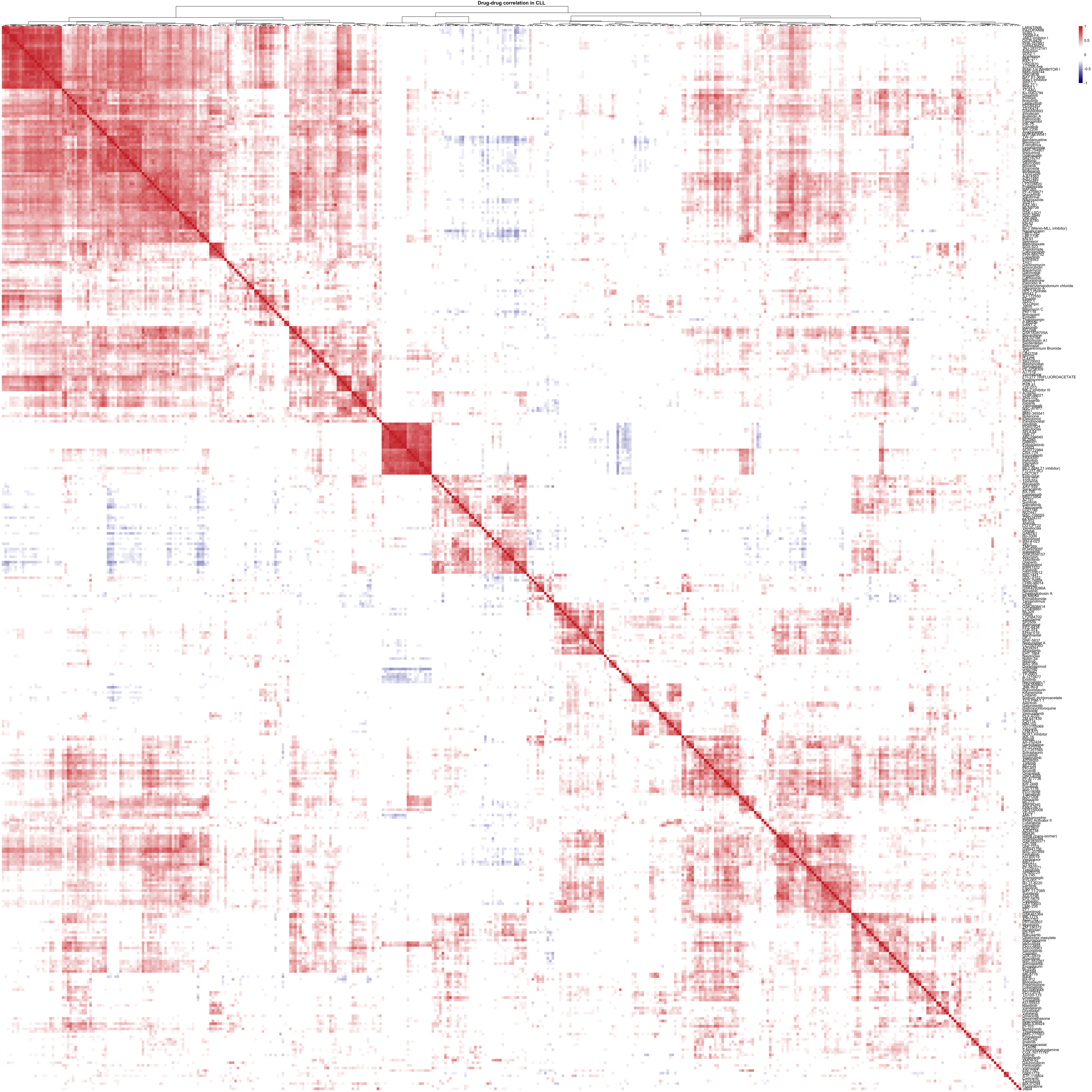
Drug-drug correlation matrix (only drugs that could produce AUC data in all samples)
viabMat <- viabMat[complete.cases(viabMat),]
corMat <- cor(t(viabMat), use = "pairwise.complete.obs")

#define color sequences
colorList <- c(colorRampPalette(c("navy", "white"))(20),
               colorRampPalette(c("white"))(10),
               colorRampPalette(c("white","firebrick3"))(20))

pheatmap(corMat, breaks = seq(-1,1,length.out = 50),
         clustering_method = "ward.D2", color = colorList,
         treeheight_row = 0, show_colnames = FALSE,
         main = "Drug-drug correlation in CLL")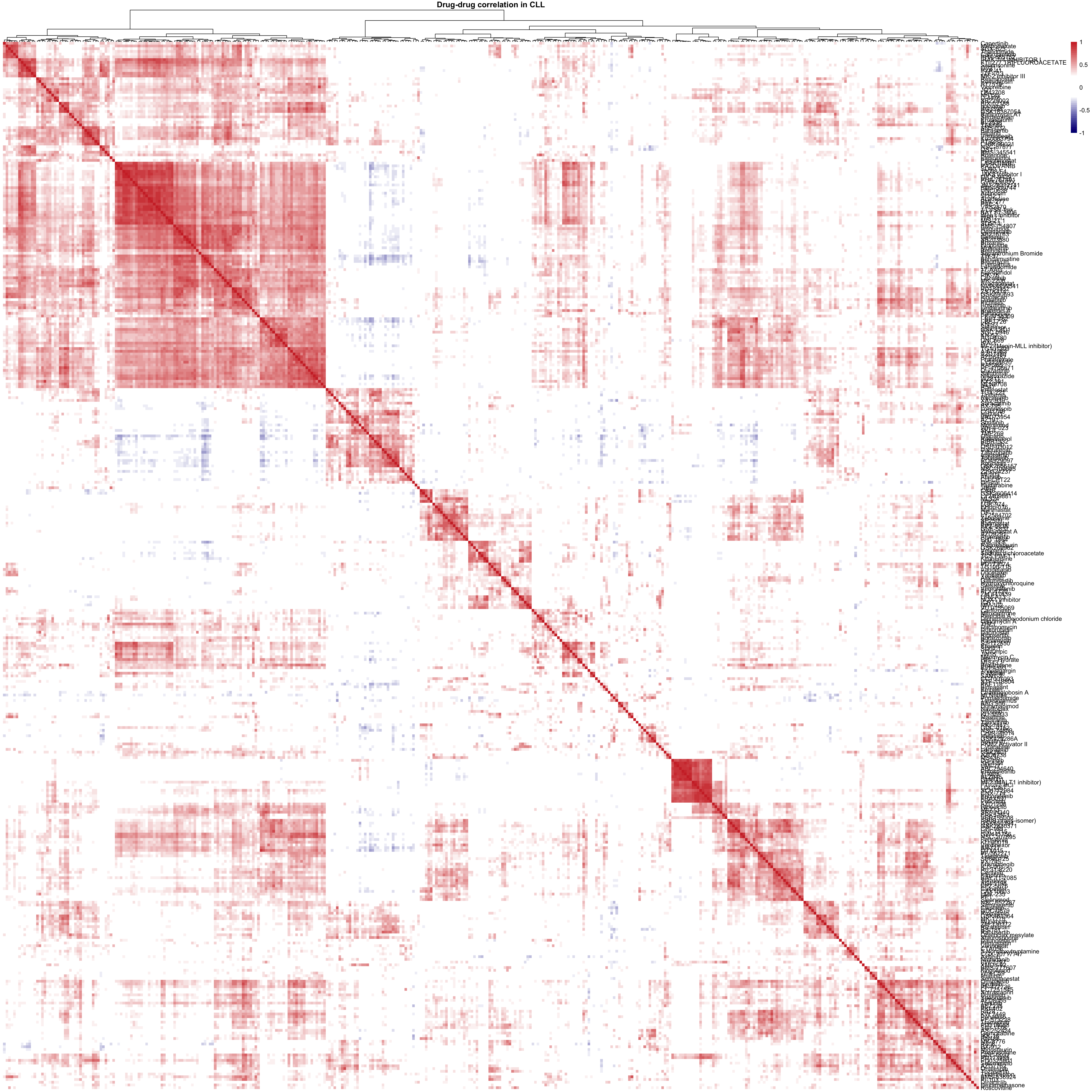
For M-CLL samples
#Prepare viability matrix
viabMat <- filter(screenData, diagnosis %in% "CLL", patientID %in% filter(patMeta, IGHV.status %in% "M")$Patient.ID) %>%
  group_by(patientID, Drug) %>% summarise(viab = mean(viab.auc, na.rm=TRUE)) %>%
  spread(key = patientID, value = "viab") %>% data.frame() %>%
  column_to_rownames("Drug") %>% as.matrix()
viabMat <- viabMat[rowSums(!is.na(viabMat))>2,]
#viabMat <- viabMat[complete.cases(viabMat),]
Drug-drug correlation matrix (all drugs, except for those that generate AUC data in less than 3 samples)
corMat <- cor(t(viabMat), use = "pairwise.complete.obs")

#define color sequences
colorList <- c(colorRampPalette(c("navy", "white"))(20),
               colorRampPalette(c("white"))(10),
               colorRampPalette(c("white","firebrick3"))(20))

pheatmap(corMat, breaks = seq(-1,1,length.out = 50),
         clustering_method = "ward.D2", color = colorList,
         treeheight_row = 0, show_colnames = FALSE,
         main = "Drug-drug correlation in CLL")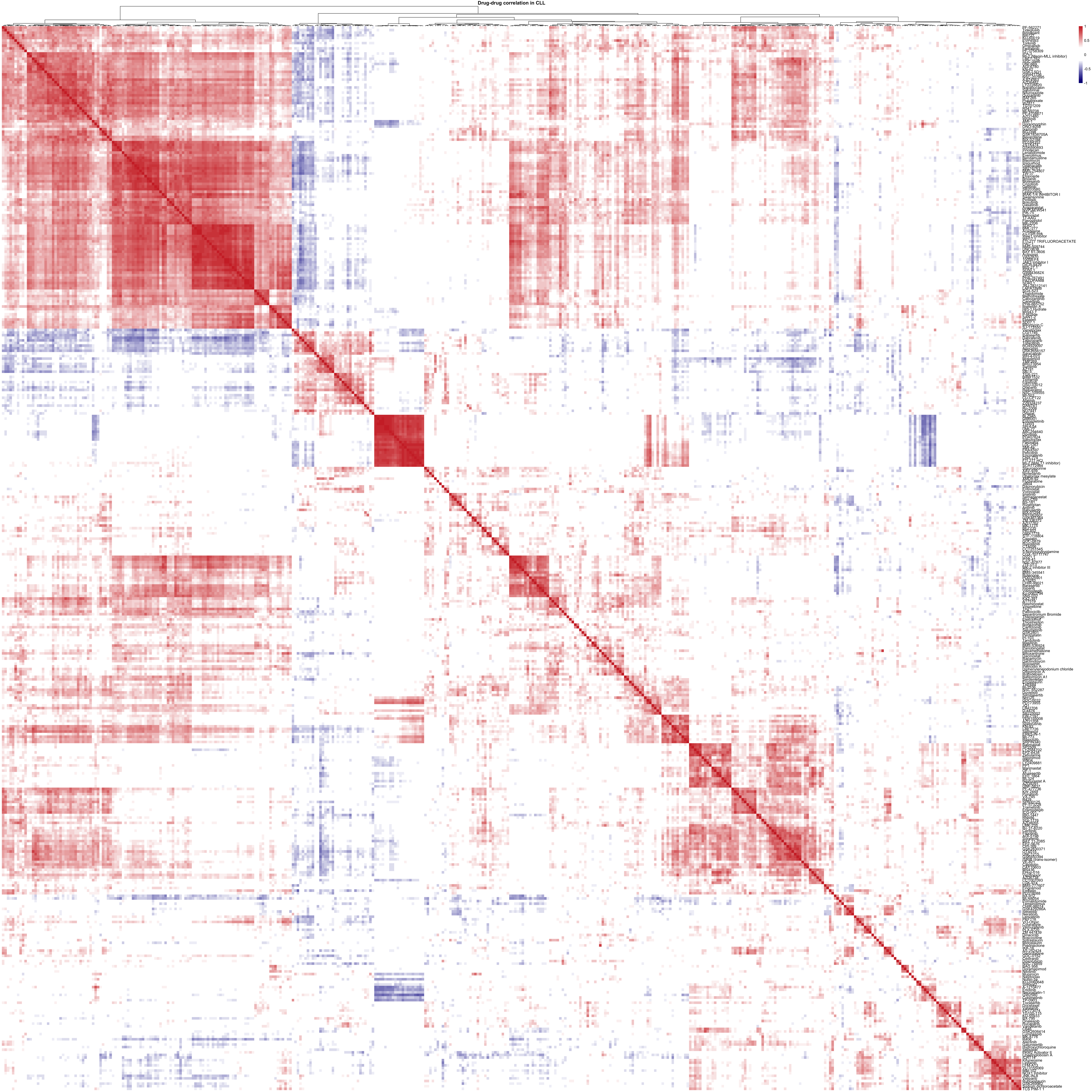
Drug-drug correlation matrix (only drugs that could produce AUC data in all samples)
viabMat <- viabMat[complete.cases(viabMat),]
corMat <- cor(t(viabMat), use = "pairwise.complete.obs")

#define color sequences
colorList <- c(colorRampPalette(c("navy", "white"))(20),
               colorRampPalette(c("white"))(10),
               colorRampPalette(c("white","firebrick3"))(20))

pheatmap(corMat, breaks = seq(-1,1,length.out = 50),
         clustering_method = "ward.D2", color = colorList,
         treeheight_row = 0, show_colnames = FALSE,
         main = "Drug-drug correlation in CLL")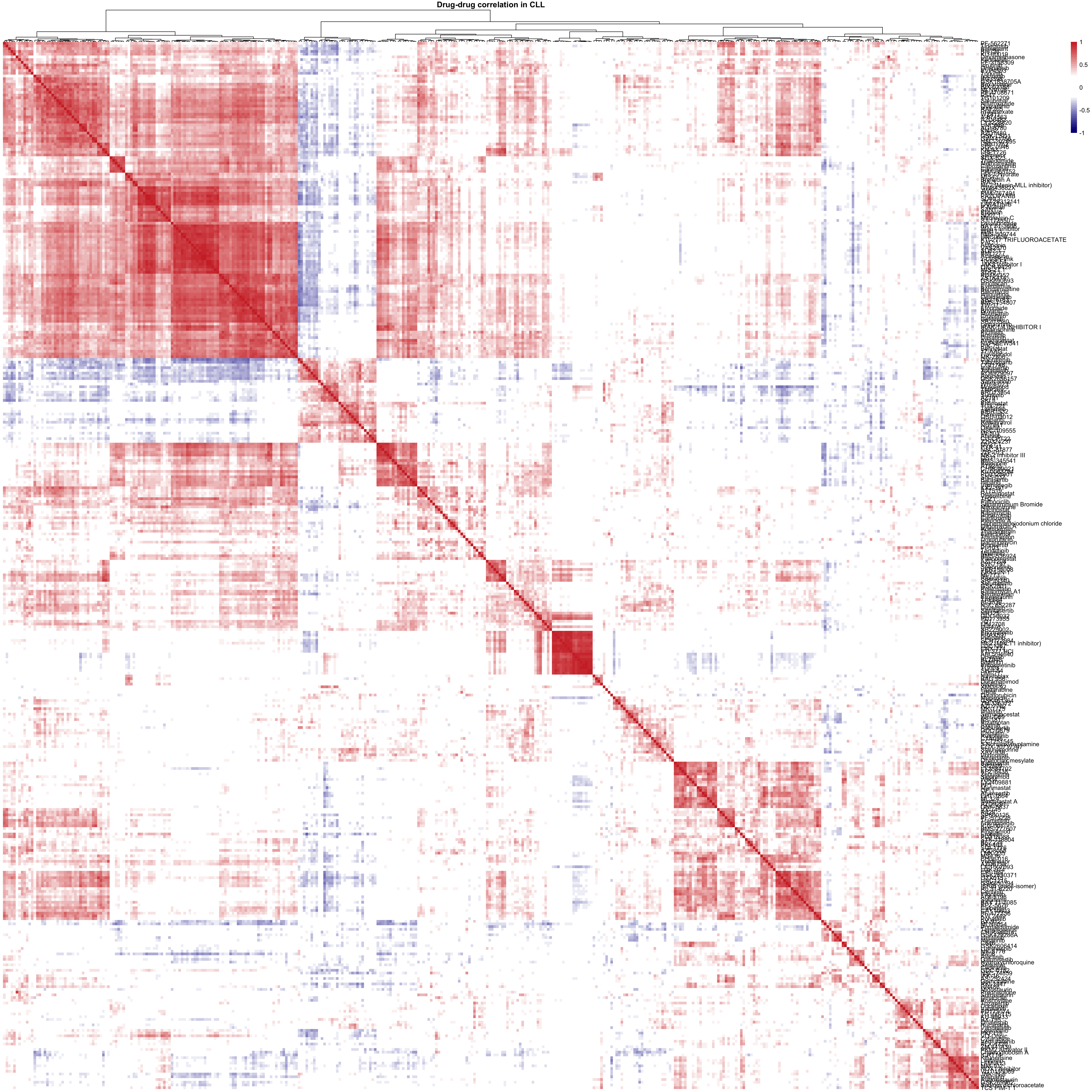
For U-CLL samples
#Prepare viability matrix
viabMat <- filter(screenData, diagnosis %in% "CLL", patientID %in% filter(patMeta, IGHV.status %in% "U")$Patient.ID) %>%
  group_by(patientID, Drug) %>% summarise(viab = mean(viab.auc, na.rm=TRUE)) %>%
  spread(key = patientID, value = "viab") %>% data.frame() %>%
  column_to_rownames("Drug") %>% as.matrix()
viabMat <- viabMat[rowSums(!is.na(viabMat))>2,]
#viabMat <- viabMat[complete.cases(viabMat),]
Drug-drug correlation matrix (all drugs, except for those that generate AUC data in less than 3 samples)
corMat <- cor(t(viabMat), use = "pairwise.complete.obs")

#define color sequences
colorList <- c(colorRampPalette(c("navy", "white"))(20),
               colorRampPalette(c("white"))(10),
               colorRampPalette(c("white","firebrick3"))(20))

pheatmap(corMat, breaks = seq(-1,1,length.out = 50),
         clustering_method = "ward.D2", color = colorList,
         treeheight_row = 0, show_colnames = FALSE,
         main = "Drug-drug correlation in U-CLL")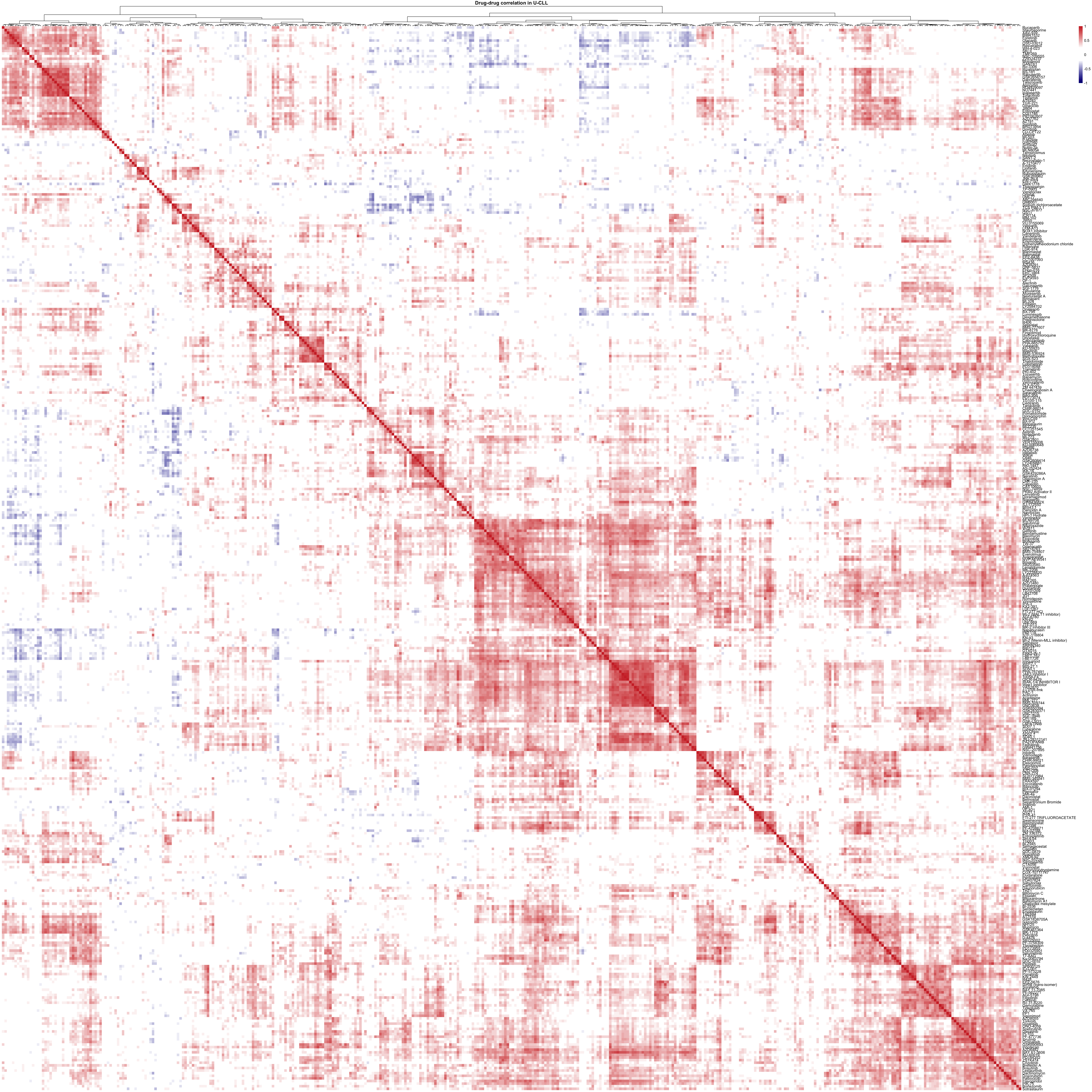
Drug-drug correlation matrix (only drugs that could produce AUC data in all samples)
viabMat <- viabMat[complete.cases(viabMat),]
corMat <- cor(t(viabMat), use = "pairwise.complete.obs")

#define color sequences
colorList <- c(colorRampPalette(c("navy", "white"))(20),
               colorRampPalette(c("white"))(10),
               colorRampPalette(c("white","firebrick3"))(20))

pheatmap(corMat, breaks = seq(-1,1,length.out = 50),
         clustering_method = "ward.D2", color = colorList,
         treeheight_row = 0, show_colnames = FALSE,
         main = "Drug-drug correlation in CLL")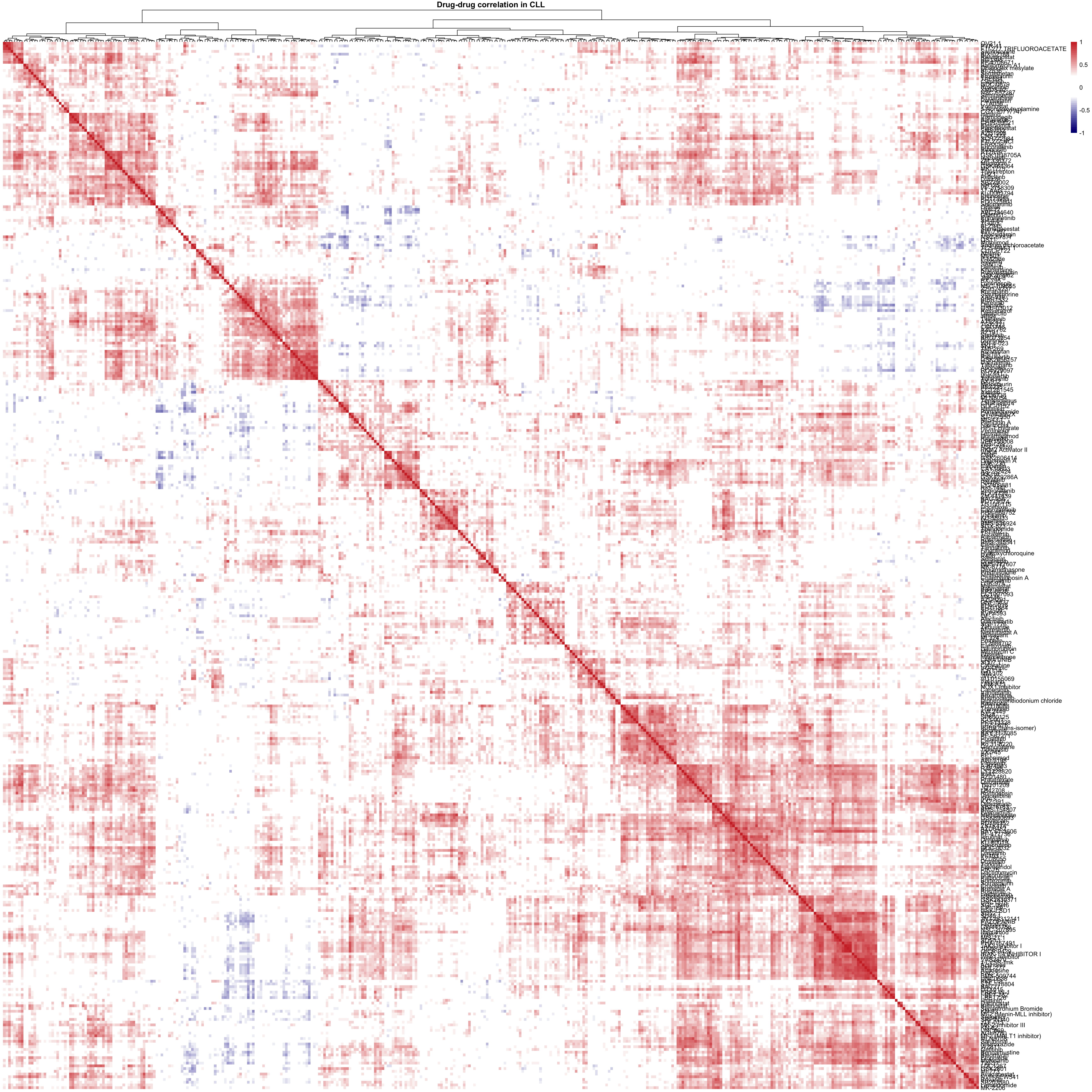
For MCL samples
Drug-drug correlation matrix (all drugs, except for those that generate AUC data in less than 3 samples)
corMat <- cor(t(viabMat), use = "pairwise.complete.obs")
pheatmap(corMat, color = colorList,
         breaks = seq(-1,1,length.out = 50), clustering_method = "ward.D2",
         treeheight_row = 0, show_colnames = FALSE,
         main = "Drug-drug correlation in MCL")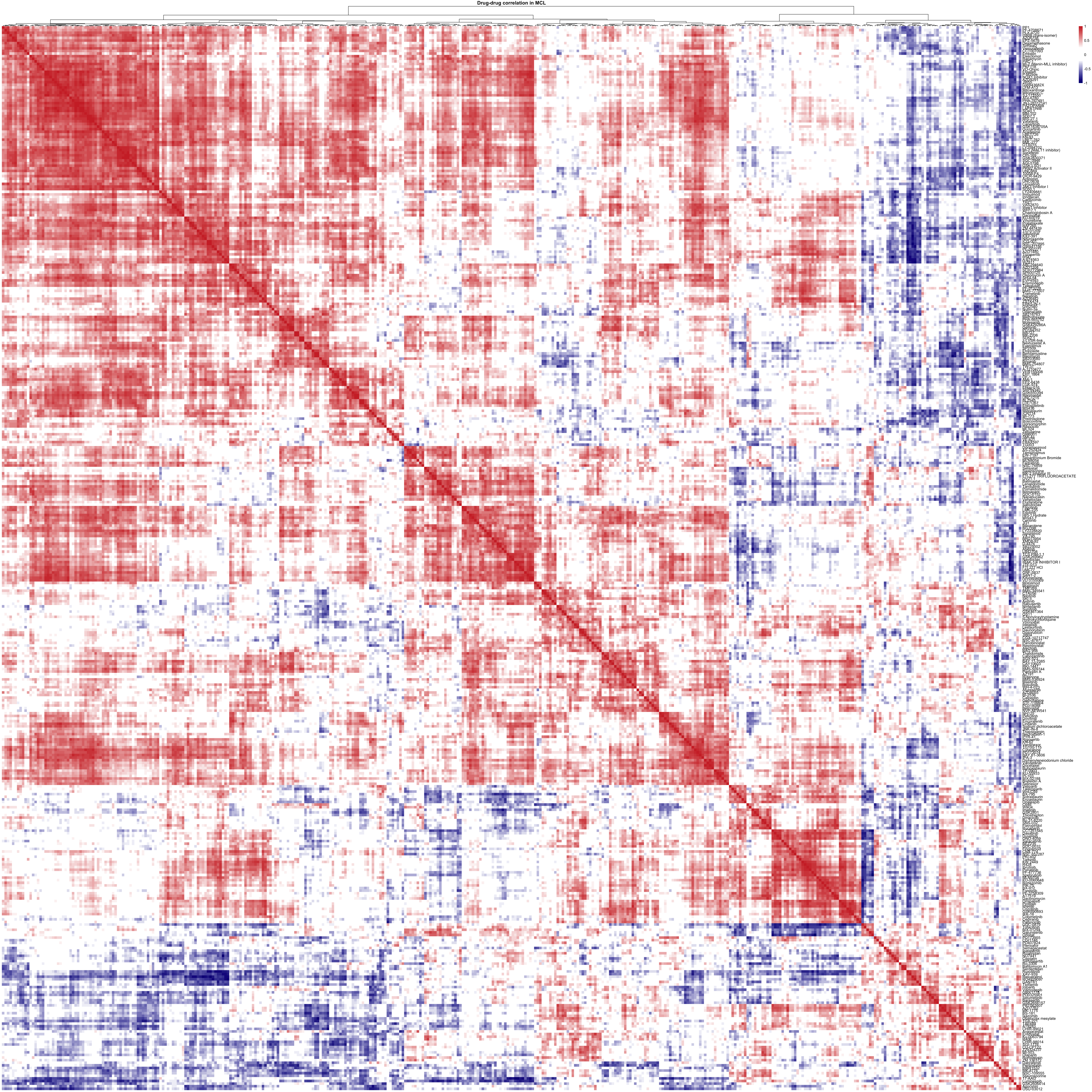
Drug-drug correlation matrix (only drugs that could produce AUC data in all samples)
viabMat <- viabMat[complete.cases(viabMat),]
corMat <- cor(t(viabMat))
pheatmap(corMat, color = colorList,
         breaks = seq(-1,1,length.out = 50), clustering_method = "ward.D2",
         treeheight_row = 0, show_colnames = FALSE,
         main = "Drug-drug correlation in MCL")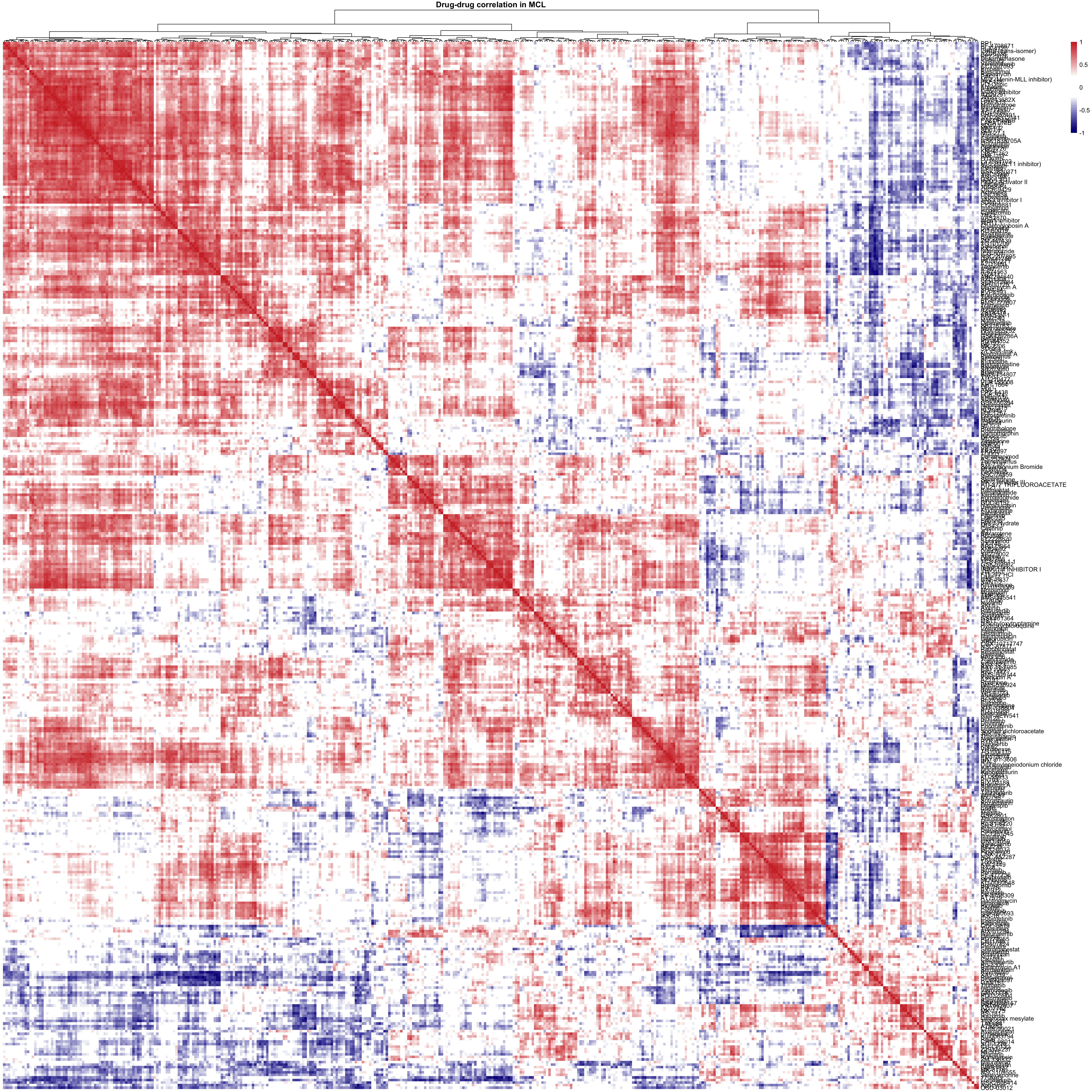
For T-PLL samples
#Prepare viability matrix
viabMat <- filter(screenData, ! Drug %in% c("DMSO","PBS"), diagnosis %in% "T-PLL") %>%
  group_by(patientID, Drug) %>% summarise(viab = mean(viab.auc, na.rm=TRUE)) %>%
  spread(key = patientID, value = "viab") %>% data.frame() %>%
  column_to_rownames("Drug") %>% as.matrix()
#viabMat <- viabMat[complete.cases(viabMat),]
viabMat <- viabMat[rowSums(!is.na(viabMat))>2,]
Drug-drug correlation matrix (all drugs, except for those that generate AUC data in less than 3 samples)
corMat <- cor(t(viabMat),use="pairwise.complete.obs")
pheatmap(corMat, color = colorList,
         breaks = seq(-1,1,length.out = 50), clustering_method = "ward.D2",
         treeheight_row = 0, show_colnames = FALSE,
         main = "Drug-drug correlation in T-PLL")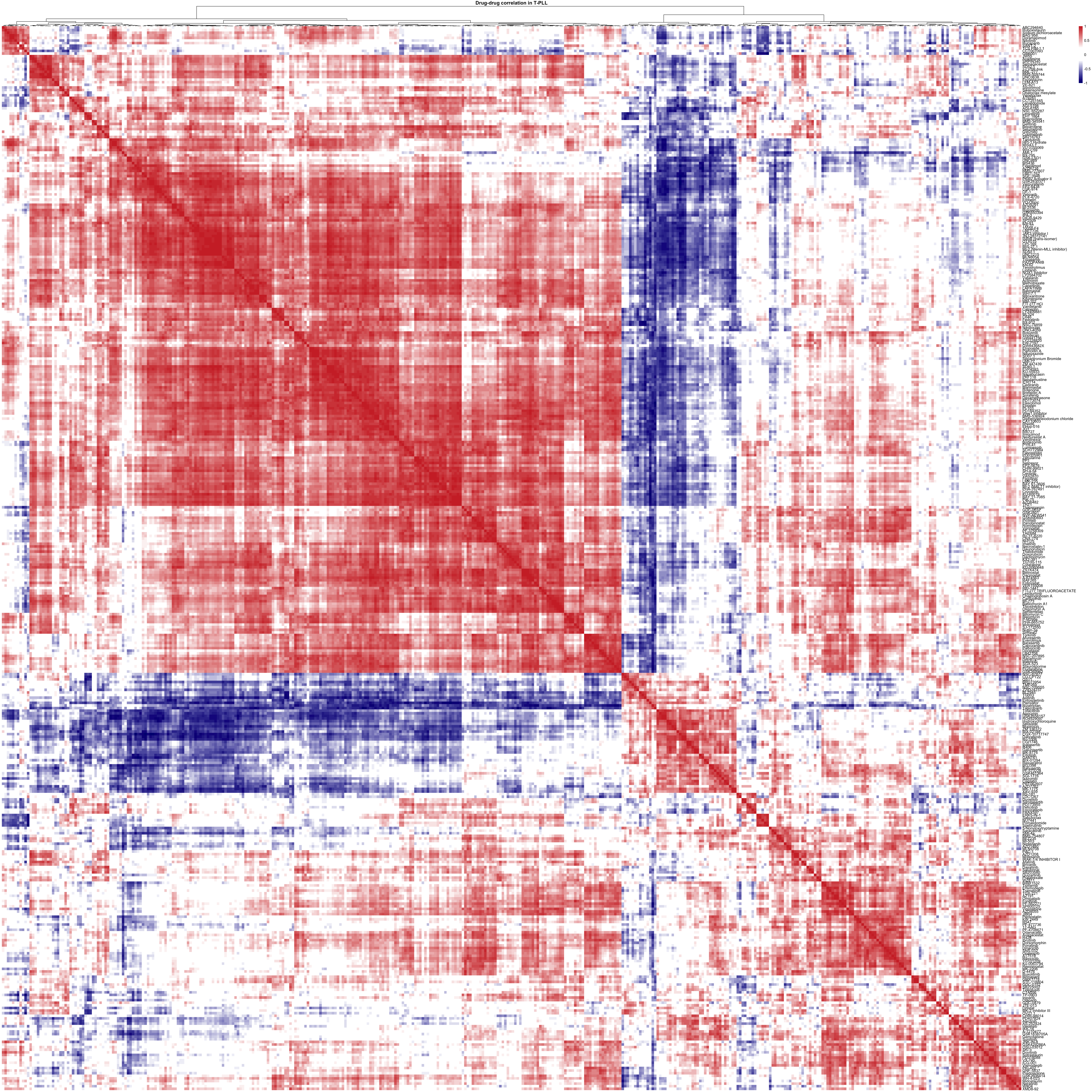
viabMat <- viabMat[complete.cases(viabMat),]
corMat <- cor(t(viabMat),use="pairwise.complete.obs")
pheatmap(corMat, color = colorList,
         breaks = seq(-1,1,length.out = 50), clustering_method = "ward.D2",
         treeheight_row = 0, show_colnames = FALSE,
         main = "Drug-drug correlation in T-PLL")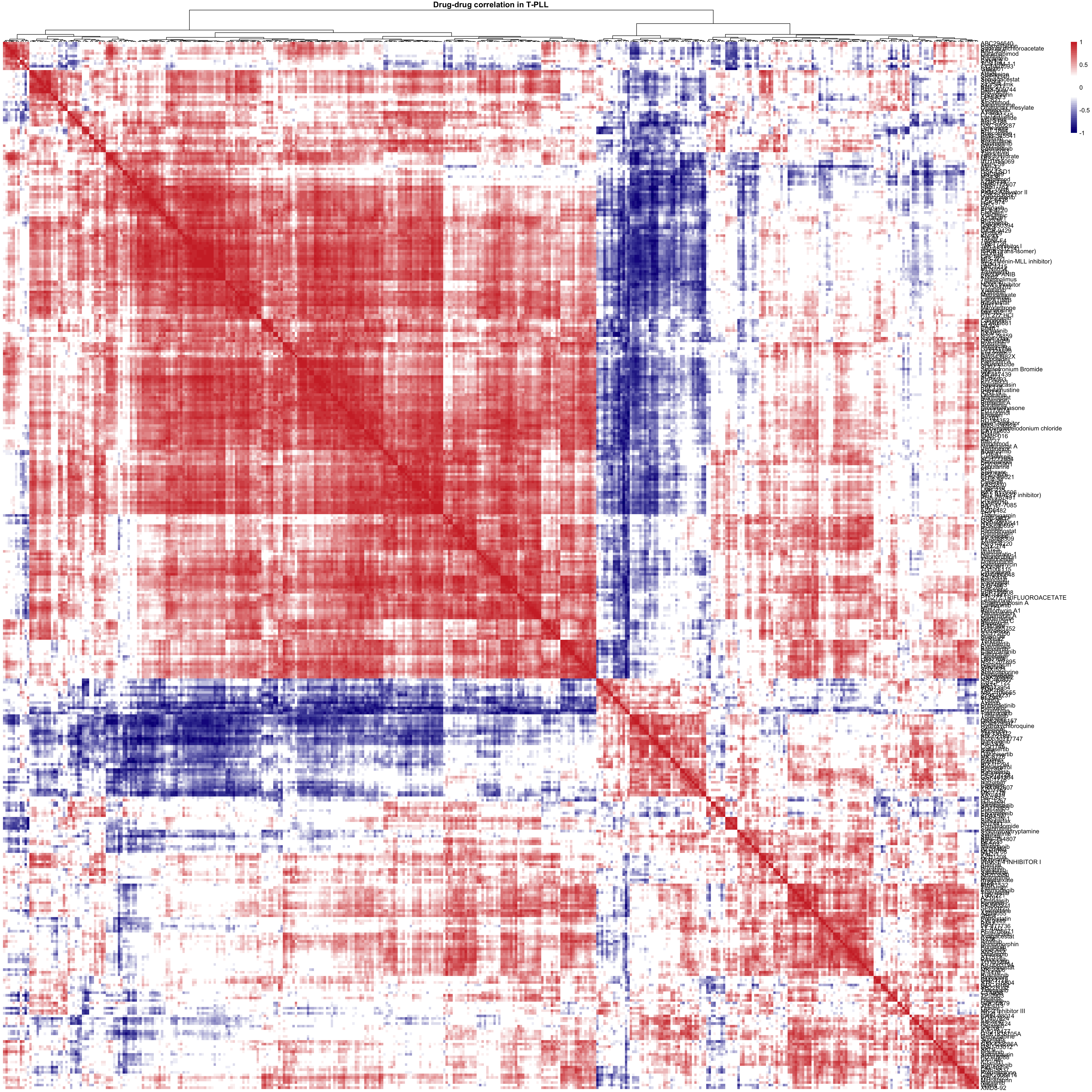
sessionInfo()R version 4.2.0 (2022-04-22)
Platform: x86_64-apple-darwin17.0 (64-bit)
Running under: macOS Big Sur/Monterey 10.16
Matrix products: default
BLAS: /Library/Frameworks/R.framework/Versions/4.2/Resources/lib/libRblas.0.dylib
LAPACK: /Library/Frameworks/R.framework/Versions/4.2/Resources/lib/libRlapack.dylib
locale:
[1] en_US.UTF-8/en_US.UTF-8/en_US.UTF-8/C/en_US.UTF-8/en_US.UTF-8
attached base packages:
[1] stats graphics grDevices utils datasets methods base
other attached packages:
[1] forcats_0.5.1 stringr_1.4.0 dplyr_1.0.9
[4] purrr_0.3.4 readr_2.1.2 tidyr_1.2.0
[7] tibble_3.1.8 tidyverse_1.3.2 limma_3.52.2
[10] readxl_1.4.0 gtable_0.3.0 ggbeeswarm_0.6.0
[13] jyluMisc_0.1.5 colorspace_2.0-3 RColorBrewer_1.1-3
[16] ggrepel_0.9.1 ggplot2_3.3.6 smallvis_0.0.0.9000
[19] Rtsne_0.16 cowplot_1.1.1 genefilter_1.78.0
[22] pheatmap_1.0.12 reshape2_1.4.4 gridExtra_2.3
[25] Biobase_2.56.0 BiocGenerics_0.42.0
loaded via a namespace (and not attached):
[1] utf8_1.2.2 shinydashboard_0.7.2
[3] tidyselect_1.1.2 RSQLite_2.2.15
[5] AnnotationDbi_1.58.0 htmlwidgets_1.5.4
[7] grid_4.2.0 BiocParallel_1.30.3
[9] maxstat_0.7-25 munsell_0.5.0
[11] ragg_1.2.2 codetools_0.2-18
[13] DT_0.23 withr_2.5.0
[15] highr_0.9 knitr_1.39
[17] rstudioapi_0.13 stats4_4.2.0
[19] ggsignif_0.6.3 MatrixGenerics_1.8.1
[21] labeling_0.4.2 git2r_0.30.1
[23] slam_0.1-50 GenomeInfoDbData_1.2.8
[25] KMsurv_0.1-5 bit64_4.0.5
[27] farver_2.1.1 rprojroot_2.0.3
[29] vctrs_0.4.1 generics_0.1.3
[31] TH.data_1.1-1 xfun_0.31
[33] sets_1.0-21 R6_2.5.1
[35] GenomeInfoDb_1.32.2 bitops_1.0-7
[37] cachem_1.0.6 fgsea_1.22.0
[39] DelayedArray_0.22.0 assertthat_0.2.1
[41] vroom_1.5.7 promises_1.2.0.1
[43] scales_1.2.0 multcomp_1.4-19
[45] googlesheets4_1.0.0 beeswarm_0.4.0
[47] sandwich_3.0-2 workflowr_1.7.0
[49] rlang_1.0.4 systemfonts_1.0.4
[51] splines_4.2.0 rstatix_0.7.0
[53] gargle_1.2.0 broom_1.0.0
[55] BiocManager_1.30.18 yaml_2.3.5
[57] abind_1.4-5 modelr_0.1.8
[59] backports_1.4.1 httpuv_1.6.5
[61] tools_4.2.0 relations_0.6-12
[63] ellipsis_0.3.2 gplots_3.1.3
[65] jquerylib_0.1.4 Rcpp_1.0.9
[67] plyr_1.8.7 visNetwork_2.1.0
[69] zlibbioc_1.42.0 RCurl_1.98-1.7
[71] ggpubr_0.4.0 S4Vectors_0.34.0
[73] zoo_1.8-10 SummarizedExperiment_1.26.1
[75] haven_2.5.0 cluster_2.1.3
[77] exactRankTests_0.8-35 fs_1.5.2
[79] magrittr_2.0.3 data.table_1.14.2
[81] reprex_2.0.1 survminer_0.4.9
[83] googledrive_2.0.0 mvtnorm_1.1-3
[85] matrixStats_0.62.0 hms_1.1.1
[87] shinyjs_2.1.0 mime_0.12
[89] evaluate_0.15 xtable_1.8-4
[91] XML_3.99-0.10 IRanges_2.30.0
[93] compiler_4.2.0 KernSmooth_2.23-20
[95] crayon_1.5.1 htmltools_0.5.3
[97] later_1.3.0 tzdb_0.3.0
[99] lubridate_1.8.0 DBI_1.1.3
[101] dbplyr_2.2.1 MASS_7.3-58
[103] BiocStyle_2.24.0 Matrix_1.4-1
[105] car_3.1-0 cli_3.3.0
[107] marray_1.74.0 parallel_4.2.0
[109] igraph_1.3.4 GenomicRanges_1.48.0
[111] pkgconfig_2.0.3 km.ci_0.5-6
[113] piano_2.12.0 xml2_1.3.3
[115] annotate_1.74.0 vipor_0.4.5
[117] bslib_0.4.0 XVector_0.36.0
[119] drc_3.0-1 rvest_1.0.2
[121] digest_0.6.29 Biostrings_2.64.0
[123] rmarkdown_2.14 cellranger_1.1.0
[125] fastmatch_1.1-3 survMisc_0.5.6
[127] shiny_1.7.2 gtools_3.9.3
[129] lifecycle_1.0.1 jsonlite_1.8.0
[131] carData_3.0-5 fansi_1.0.3
[133] pillar_1.8.0 lattice_0.20-45
[135] KEGGREST_1.36.3 fastmap_1.1.0
[137] httr_1.4.3 plotrix_3.8-2
[139] survival_3.4-0 glue_1.6.2
[141] png_0.1-7 bit_4.0.4
[143] stringi_1.7.8 sass_0.4.2
[145] blob_1.2.3 textshaping_0.3.6
[147] caTools_1.18.2 memoise_2.0.1