Working with Image Data in R

Based on Chapter 11 of “Modern Statistics for Modern Biology”

Wolfgang Huber

2023-03-23

Setup and resources

GitHub repo: please clone
https://github.com/wolfganghuber/WorkingWithImageData

Rendered version of the demo:
https://www.huber.embl.de/users/whuber/2304-Imaging-Data-in-R/demo.html

Talk slides (PDF):
https://www.huber.embl.de/users/whuber/2304-Imaging-Data-in-R/talk.pdf

Additional resources:
https://www.huber.embl.de/users/whuber/2304-Imaging-Data-in-R/resources/

ffmpeg:
https://ffmpeg.org or from your package manager

Install the needed R packages

pkgNeed = c("knitr", "dplyr", "ggplot2", "tidyr", "purrr", "devtools", "reshape2", "stringr",
            "terrainr", "imagefx", "dill/beyonce", "EBImage") 
pkgInst = installed.packages()[, 1]
if (!("BiocManager" %in% pkgInst)) install.packages("BiocManager")
todo = !(stringr::str_split_i(pkgNeed, "/", -1) %in% pkgInst)
if (any(todo)) BiocManager::install(pkgNeed[todo])

Download example data files. Please setwd to the top directory of the WorkingWithImageData repository

url   = "https://www.huber.embl.de/users/whuber/2304-Imaging-Data-in-R/resources/"
files = c("eakKfY5aHmY.mp4", "fvec.RData", "murmuration-flow.mp4", sprintf("tile%03d.tiff", 1:4))
dest  = "resources"
if (!dir.exists(dest)) 
  dir.create(dest)
for (f in files) {
  d = file.path(dest, f)
  if (!file.exists(d))
    download.file(paste0(url, f), d)
}

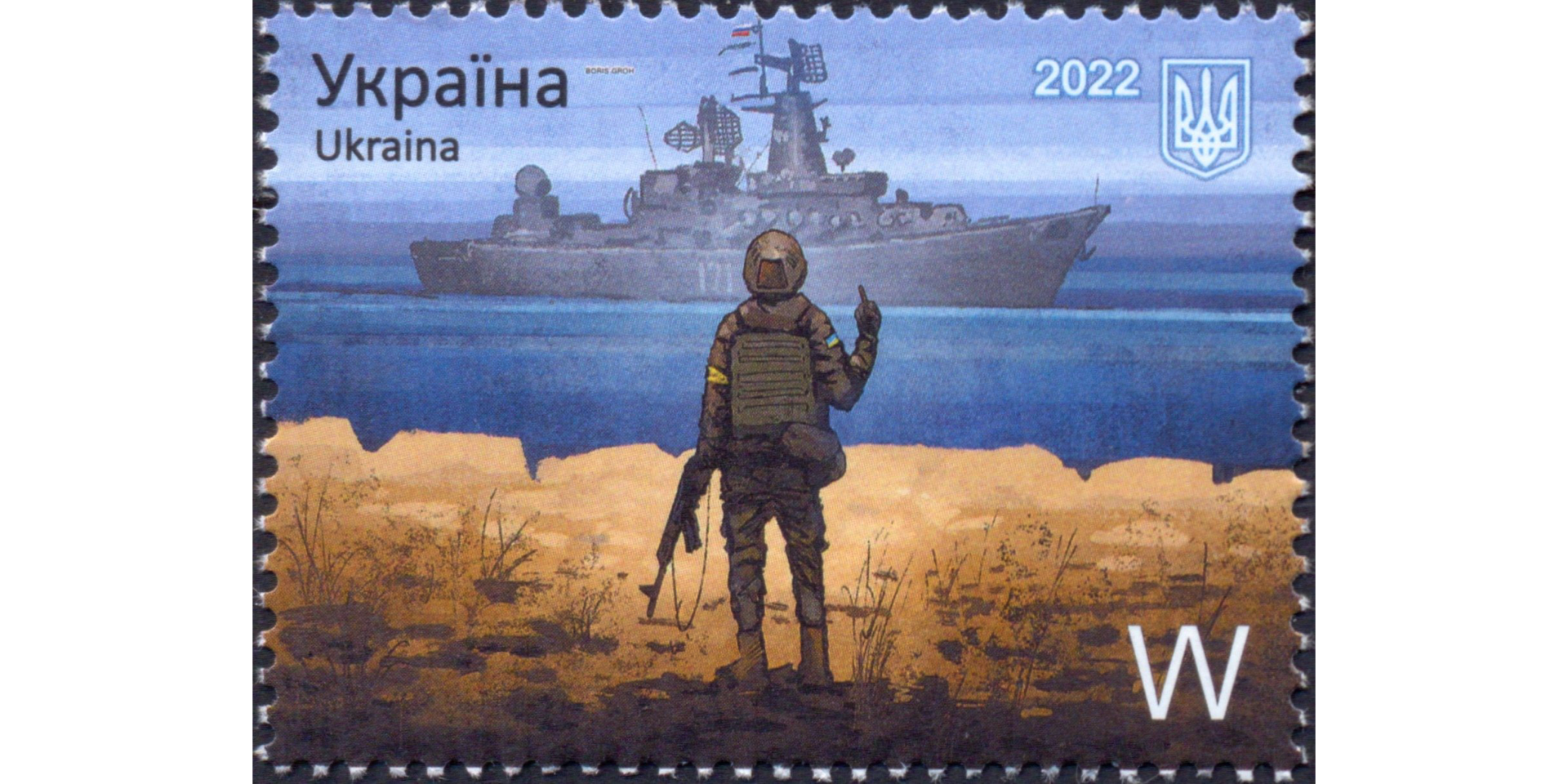
Reading and displaying an image

library("EBImage")
idi = readImage("fig/Stamp_of_Ukraine_s1985.jpg")
display(idi)

Algebraic computations

x = 1 - idi
display(x)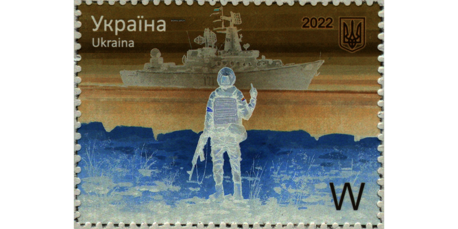

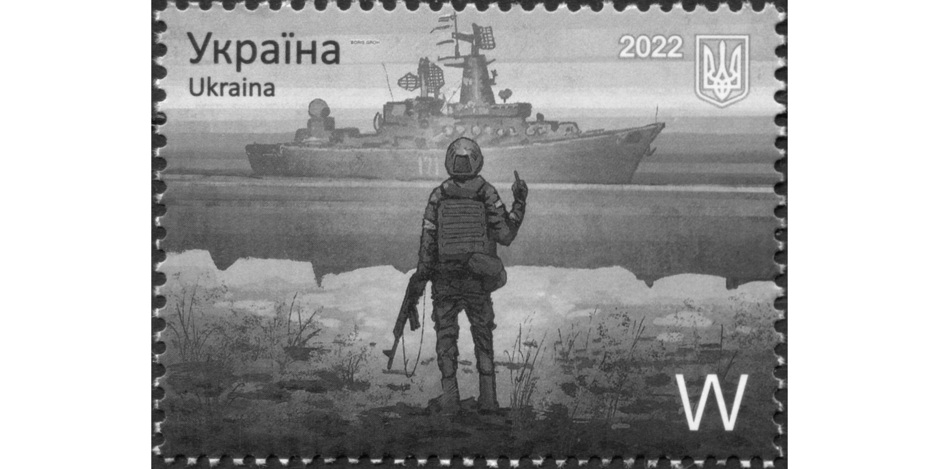
Convert into a greyscale image

idigr = (idi[,,1] + idi[,,2] + idi[,,3]) / 3    # could use `apply`; this is a bit faster
colorMode(idigr) = "grayscale"
display(idigr)

Histogram

hist(idigr)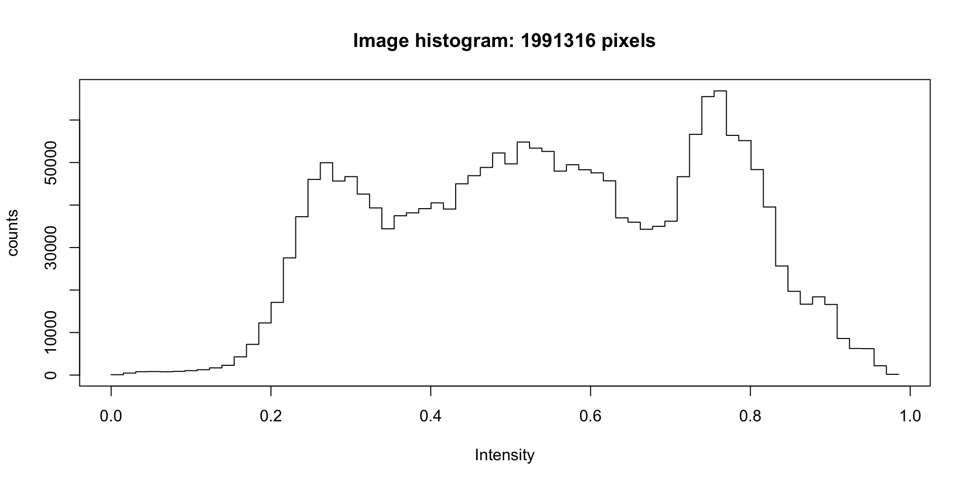

Algebraic computations

x = idigr * 2
display(x)

Computations. An image is just an array

x = idigr ^ (1/3)
display(x)

Thresholding

x = idigr > quantile(idigr, prob = 0.25)
display(x)

Transpose

x = EBImage::transpose(idi)
display(x)

Rotate

x = EBImage::rotate(idi, angle = 30)
display(x)

Translate

x = translate(idi, v = c(40, 70))
display(x)

Flip: vertical reflection

x = flip(idi)
display(x)

Flop: horizontal reflection

x = flop(idi)
display(x)

Subsetting (‘cropping’)

m = idi[800:1000, 420:560, ]
display(m)

Stitching

files = dir("resources", pattern = "^tile.*.tiff$", full.names = TRUE)
files

[1] "resources/tile001.tiff" "resources/tile002.tiff" "resources/tile003.tiff"
[4] "resources/tile004.tiff"

tiles = lapply(files, readImage) 
tiles[[1]]

Image 
  colorMode    : Color 
  storage.mode : double 
  dim          : 1920 1299 3 
  frames.total : 3 
  frames.render: 1 

imageData(object)[1:5,1:6,1]
          [,1]      [,2]      [,3]      [,4]      [,5]      [,6]
[1,] 0.9882353 0.9882353 0.9882353 0.9882353 0.9882353 0.9882353
[2,] 0.9882353 0.9882353 0.9882353 0.9882353 0.9882353 0.9882353
[3,] 0.9882353 0.9882353 0.9882353 0.9882353 0.9882353 0.9882353
[4,] 0.9882353 0.9882353 0.9882353 0.9882353 0.9882353 0.9882353
[5,] 0.9882353 0.9882353 0.9882353 0.9882353 0.9882353 0.9882353

for (x in tiles) display(x)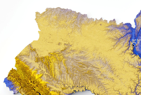

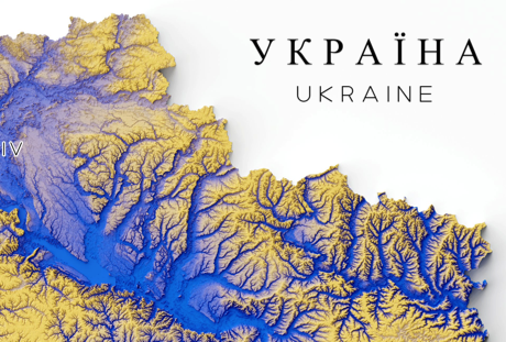
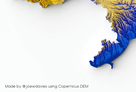
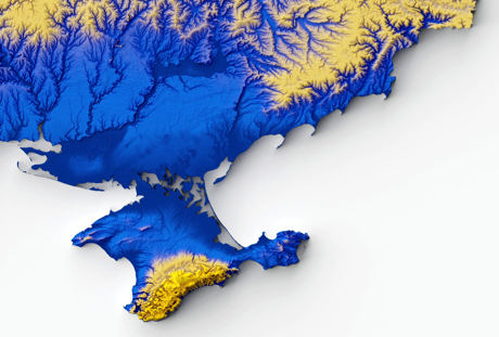
Thanks to Joe Davies (@joewdavies) for providing the image.

sx = dim(tiles[[1]])[1]    # in practice, look at all tiles and do the gymnastics as necessary  
sy = dim(tiles[[1]])[2]    
combined = Image(NA_real_, dim = c(2 * sx, 2 * sy, 3), colormode = "color")
combined[     1:sx    ,      1:sy,     ] = tiles[[1]] 
combined[(sx+1):(2*sx),      1:sy,     ] = tiles[[2]] 
combined[     1:sx    , (sy+1):(2*sy), ] = tiles[[3]]
combined[(sx+1):(2*sx), (sy+1):(2*sy), ] = tiles[[4]]
display(combined)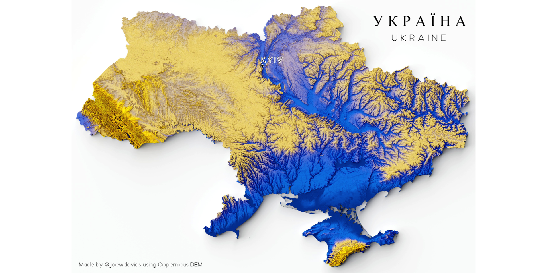

Integration with base R, dplyr, ggplot2

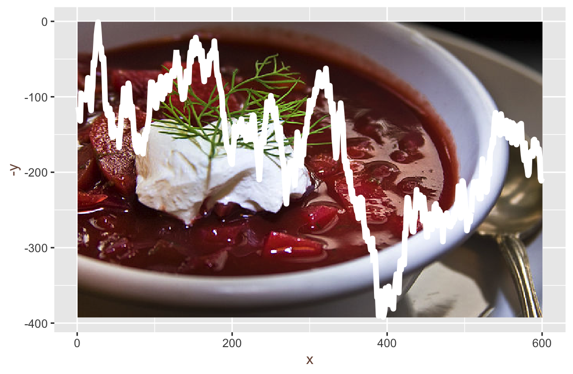
borscz = readImage("fig/borscz_1.jpg")

image(borscz)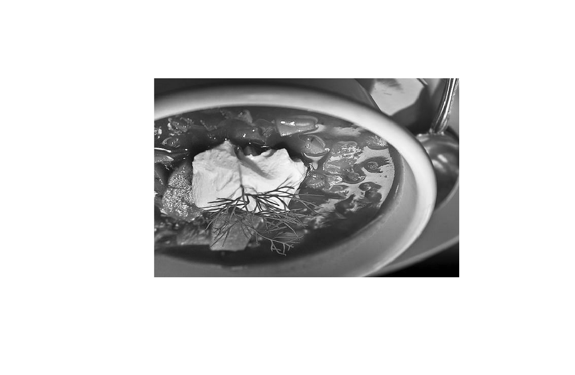

Credit: https://en.wikipedia.org/wiki/Borscht CC BY 2.0 Liz West from Boxborough, MA

library("ggplot2")
library("dplyr")
library("reshape2")  # for melt
library("terrainr")  # for geom_spatial_rgb

# Convert 3d array (x * y * RGB-colors) into a tidy dataframe, one row per pixel
array2df = function(x)
  melt(x[,,1]) |> 
    full_join(melt(x[,,2]), by = c("Var1", "Var2")) |>  
    full_join(melt(x[,,3]), by = c("Var1", "Var2")) |> 
    `colnames<-`(c("x", "y", "r", "g", "b")) 
borsczdf = array2df(borscz) 

ggplot(borsczdf, aes(x = x, y = -y, r = r, g = g, b = b)) + 
  geom_spatial_rgb()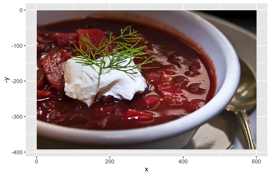

avcol = with(borsczdf, rgb(median(r), median(g), median(b)))
avcol

[1] "#785343"

rw = tibble(x = seq_len(dim(borscz)[1]),
            y = cumsum(rnorm(length(x))) |> scales::rescale(c(1, dim(borscz)[2])))
ggplot(borsczdf, aes(x = x, y = -y)) + 
  geom_spatial_rgb(aes(r = r, g = g, b = b)) +
  geom_line(data = rw, col = "white", lwd = 2) +
  theme(text = element_text(color = avcol))

Segmentation, object feature extraction and classification

Read an image

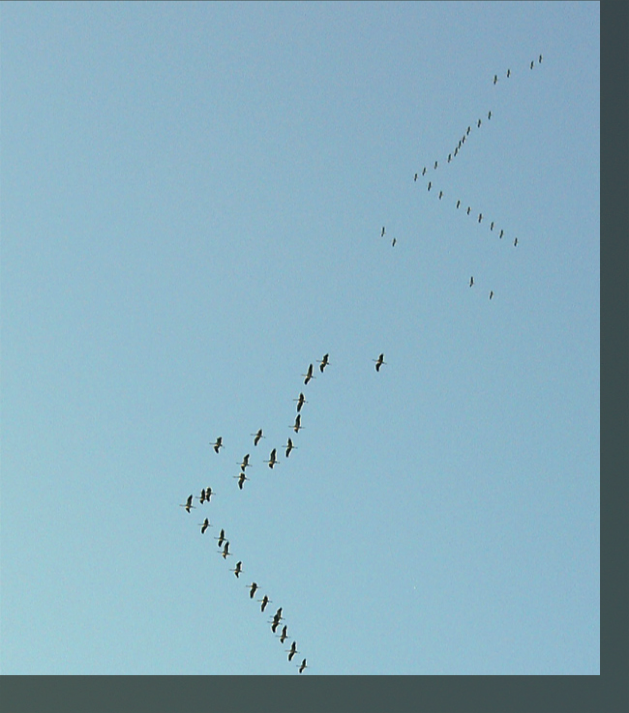
grus = readImage("fig/Grus_grus_flocks.jpg")  # common crane (Kranich, кран). Source: Wikipedia
display(grus)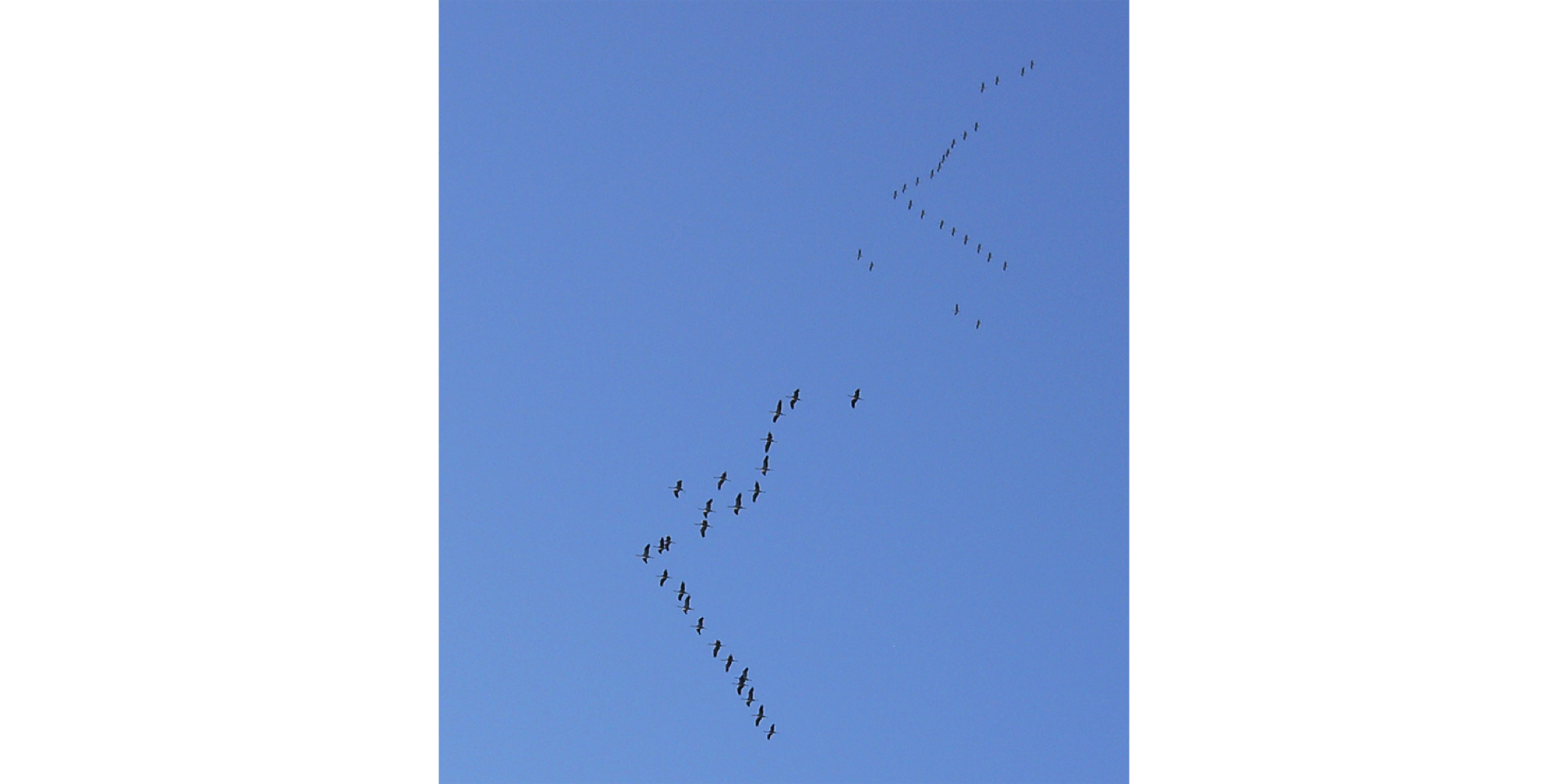

Intensity histogram, by color (RGB)

hist(grus)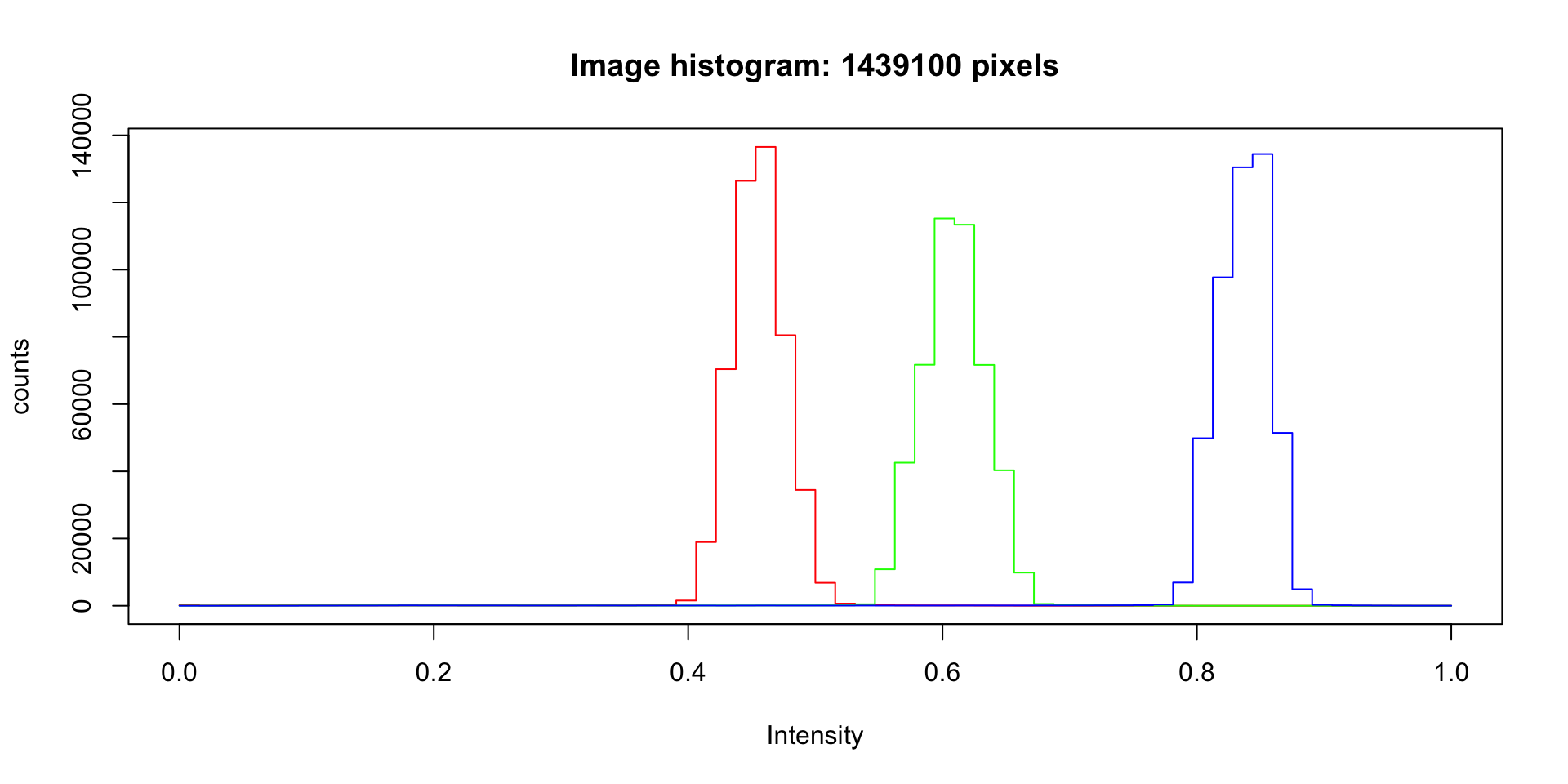

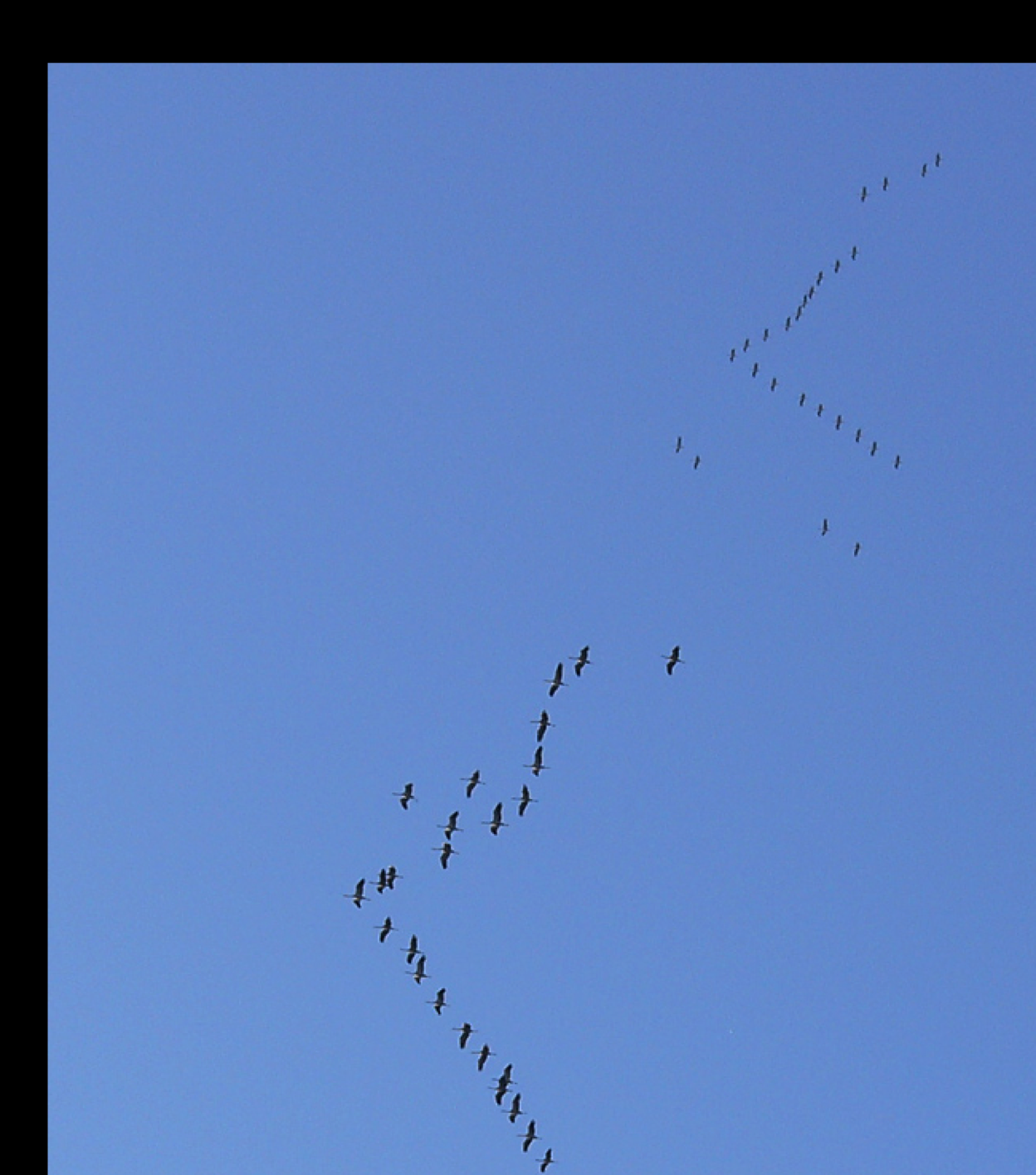
Very simple segmentation: every pixel that’s not very blue is a bird pixel

grus_fg = (grus[,,3] < 0.7) 
colorMode(grus_fg) = "grayscale"
display(grus_fg)

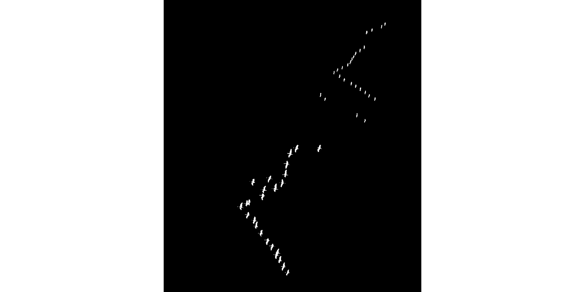
Find connected components. Intention: each is a separate object of interest (i.e., a bird)

connCompID = bwlabel(grus_fg)
display(colorLabels(connCompID))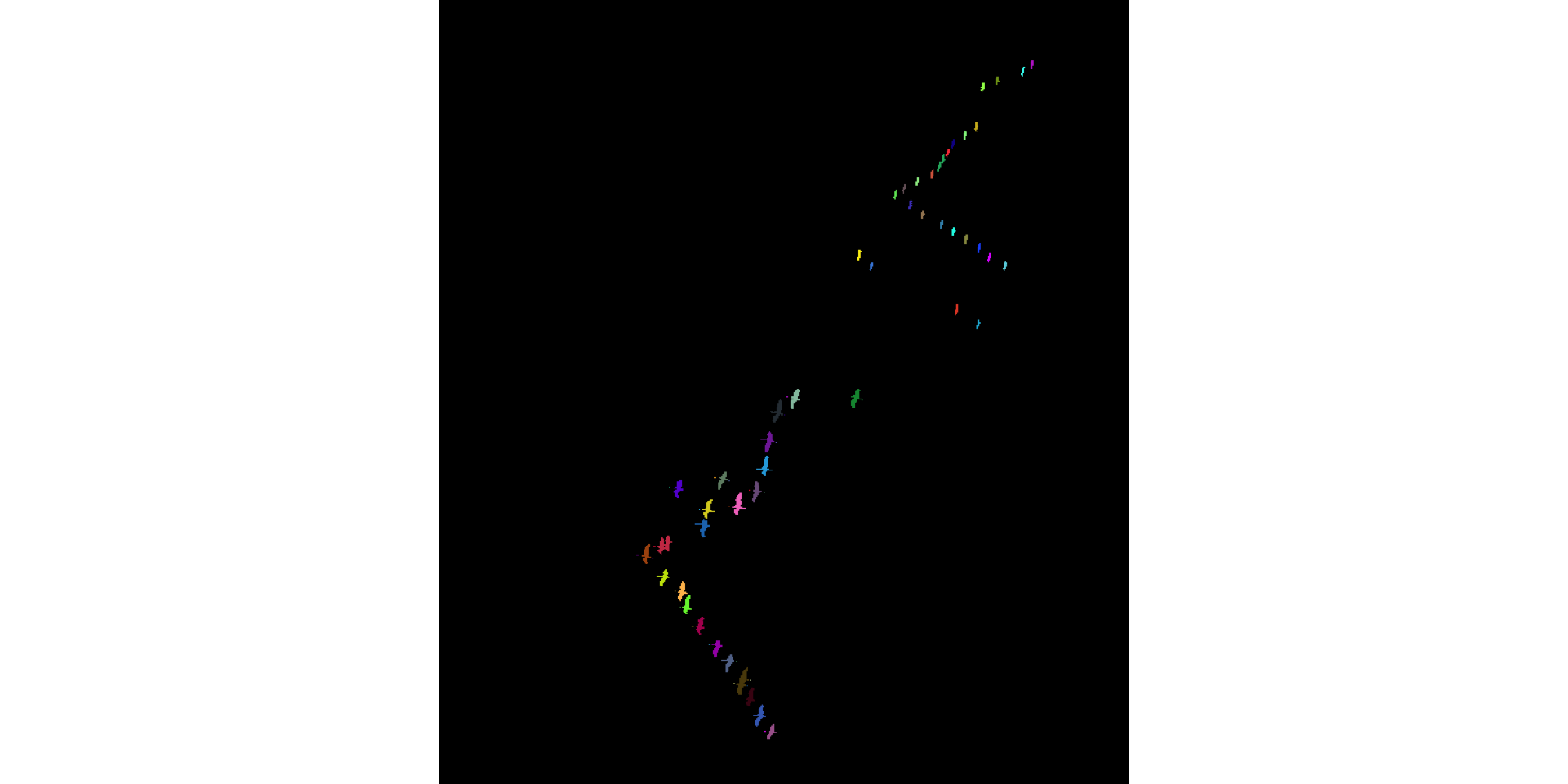

Some heads are cut off due to misclassification of bright-colored neck as sky \(\to\) small objects. Refine: eliminate such small objects. Bird bodies without necks and heads are good enough for us, for now.

connCompSize = table(connCompID) 
connCompSize

connCompID
     0      1      2      3      4      5      6      7      8      9     10 
477224     20     17     20     25     20     20     21     18     40     21 
    11     12     13     14     15     16     17     18     19     20     21 
    17     18     16     21     20     20     20     23     19     22     20 
    22     23     24     25     26     27     28     29     30     31     32 
    20     18     24     20     86     83      2     98      1      1     91 
    33     34     35     36     37     38     39     40     41     42     43 
     1     85     67      2     81      1     79      1      1      1    101 
    44     45     46     47     48     49     50     51     52     53     54 
    81      1      1     81    123     80      2      2      1     70     78 
    55     56     57     58     59     60     61     62     63     64     65 
     1     74      1     69      2     75      2     74      1    128      1 
    66     67     68     69     70     71 
     2      1     78     88     55      2 

hist(sqrt(connCompSize[-1]), breaks = 25)

bad = names(connCompSize)[connCompSize < 4]
bad

 [1] "28" "30" "31" "33" "36" "38" "40" "41" "42" "45" "46" "50" "51" "52" "55"
[16] "57" "59" "61" "63" "65" "66" "67" "71"

connCompID[ connCompID %in% as.integer(bad) ] = 0L
display(colorLabels(connCompID))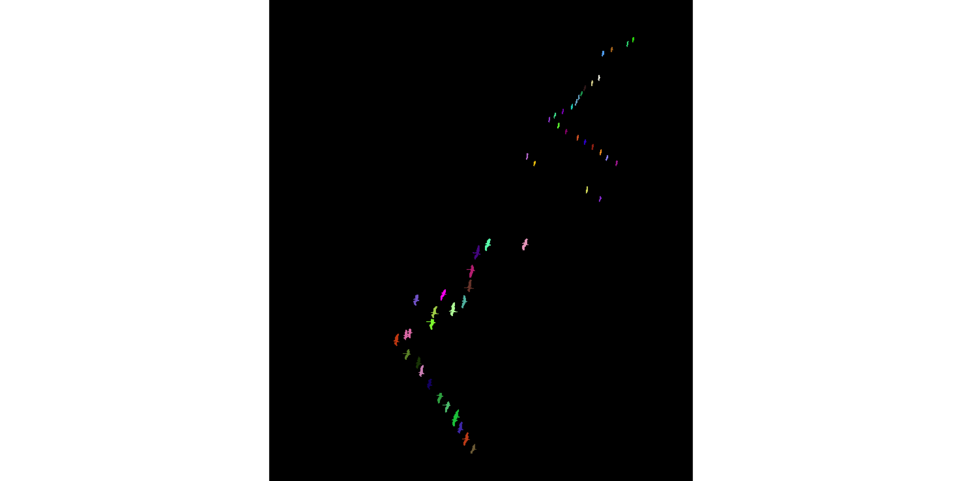

Count the number of birds. (Object “0” is the sky.)

ids = unique(as.vector(connCompID)) |> setdiff("0")
length(ids)

[1] 48

Extract their coordinates (center of mass), and any other statistic we might care about.

library("dplyr")
birds = lapply(ids, function(i) {
  w = which(connCompID == as.integer(i), arr.ind = TRUE)
  tibble(
    x = mean(w[, 1]), 
    y = mean(w[, 2]), 
    size = nrow(w),
    phi = prcomp(w)$rotation[,1] |> (\(x) atan(x[1] / x[2]))())
}) |> bind_rows() 
birds[1:3, ]

# A tibble: 3 × 4
      x     y  size    phi
  <dbl> <dbl> <int>  <dbl>
1  559.  61.3    20 -0.138
2  550.  67.8    17 -0.208
3  526.  76.4    20 -0.166

library("beyonce")
ggplot(birds, aes(x = x, y = -y, col = sqrt(size))) + geom_point() +
  scale_color_gradientn(colors = beyonce_palette(72, 21, type = "continuous")) + coord_fixed()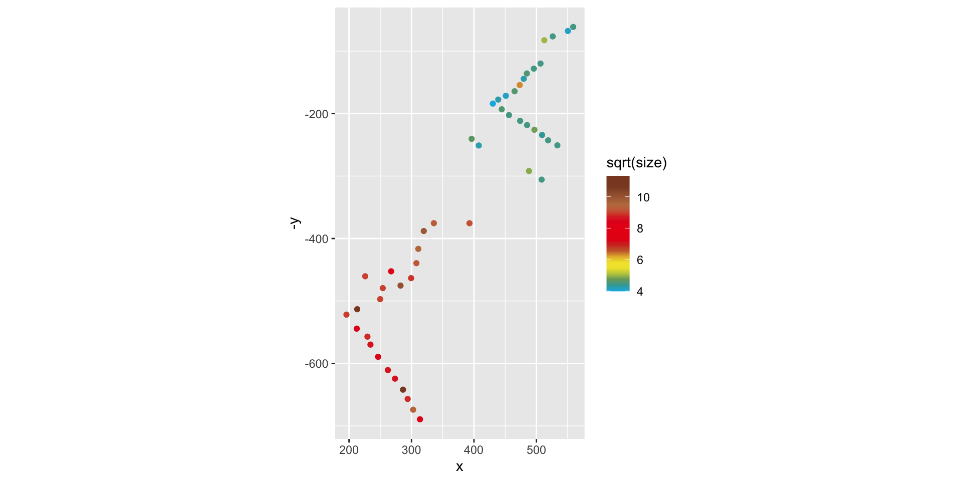

Optical flow analysis on a movie of bird murmuration

This video is by dylan.winter@virgin.net, and I got it via Youtube.

Use ffmpeg to extract the individual frames from time period 1:35 - 1:57 and store them as png files.

ffmpeg -ss 00:01:35 -t 00:01:57 -i resources/eakKfY5aHmY.mp4 frames/murm-%04d.png

Use EBImage::readImages to read into 4D array: \(n_x\times n_y\times n_{\text{colors}}\times n_{\text{timepoints}}\).

library("EBImage")
frames = dir("frames", full.names = TRUE) 
mov = readImage(frames[1:500])   # only 1:500 to save time/space, good enough for demo
dim(mov)
# [1]  1280  720    3  500

Apply Optical Flow—basically, simple linear algebra / analysis—to detect and measure local velocities of image content

trsf = function(x, y) {
  rv = atan2(y, x) / pi * 180
  ifelse(rv <= (-175), rv+360, rv)
}

vec |> 
  dplyr::filter(abs(vx) + abs(vy) >= 2) |>
  mutate(time = cut(t, 4),
         angle = trsf(vx, vy)) |>
  ggplot(aes(x = angle))  +
    coord_polar(theta = "x", start = 95/180*pi, direction = -1) +
    geom_histogram(binwidth = 15, center = 0) +
    scale_x_continuous(breaks = seq(-180, 180, by = 15), expand = c(0, 0)) + 
    facet_wrap(vars(time), ncol = 2)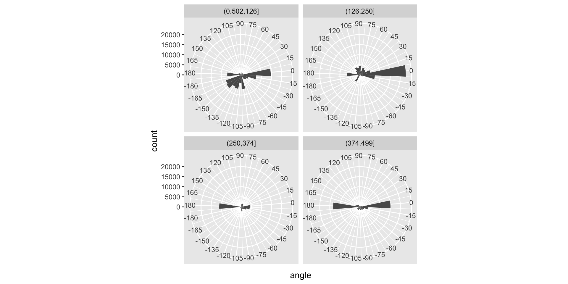

How does optical flow work?

display(grus)                     # time point 1
grus2 = translate(grus, c(30, 40))
display(grus2)                    # (simulated) time point 2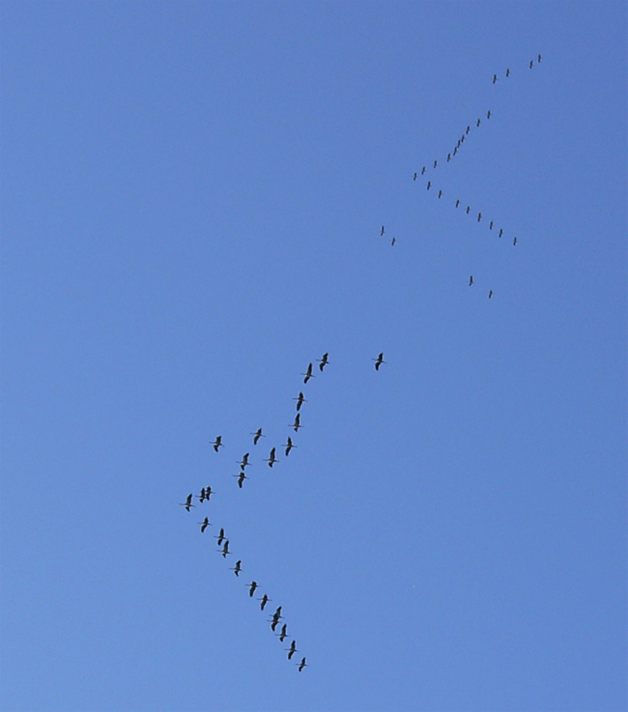

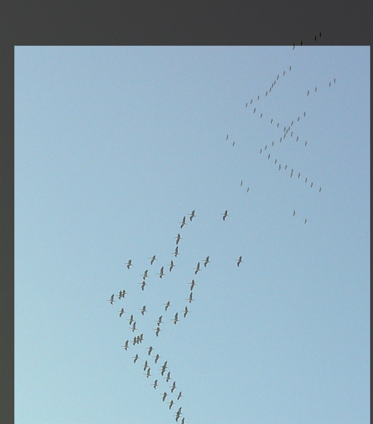
display(normalize(grus + grus2))
display(normalize(grus + translate(grus2, c(-5, 40))))
display(normalize(grus + translate(grus2, c(-30, -39))))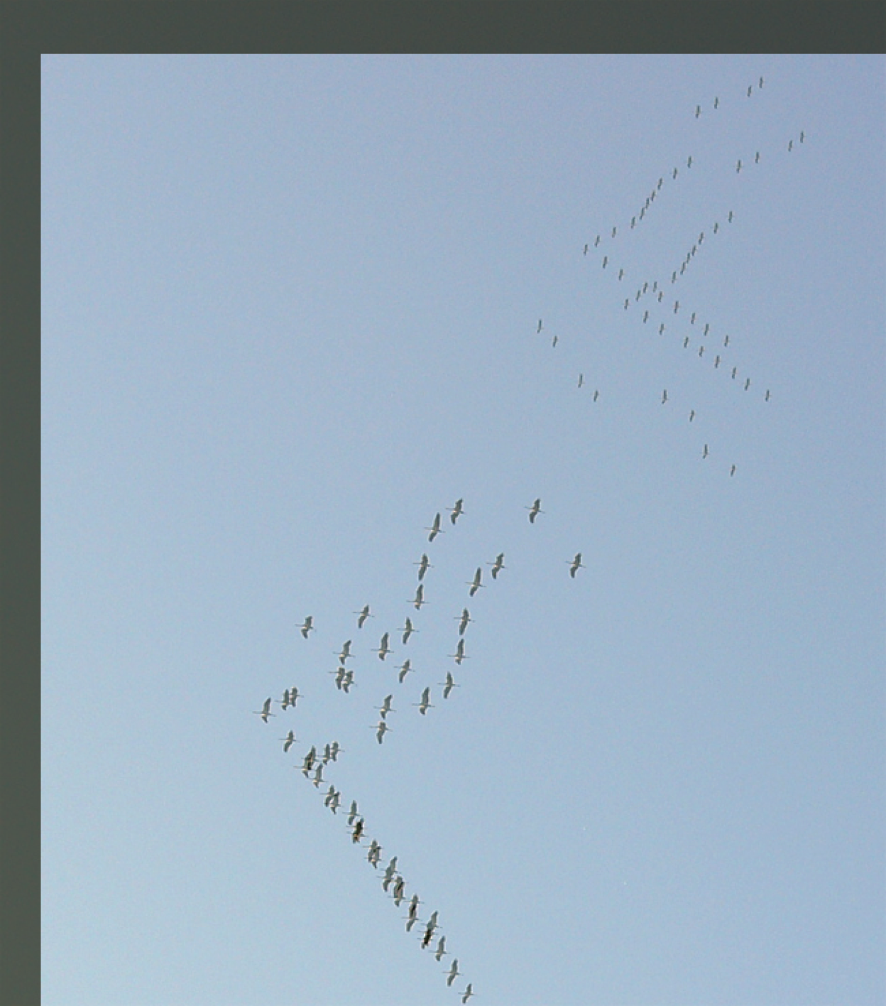

Try all possible translations of grus2 and find the one that leads to maximal overlap (correlation) with grus. imagefx::xcorr3d does this efficiently using FFT.

Full code for the bird murmuration example

# I first tried to download the video file with
youtube-dl "https://www.youtube.com/watch?v=eakKfY5aHmY"  
# but this resulted in the error message also reported here https://stackoverflow.com/questions/75495800/error-unable-to-extract-uploader-id-youtube-discord-py
# So I followed the top-voted reply there, and ran 
python3 -m pip install --force-reinstall https://github.com/yt-dlp/yt-dlp/archive/master.tar.gz
yt-dlp "https://www.youtube.com/watch?v=eakKfY5aHmY"

# The video has 25 frames per second. Some of the interesting segments are: 0:18-0:31, 1:21-1:33, 1:34-1:57, 2:10-2:32, 3:34-3:46
# I used the following to extract the frames from time period 1:35 - 1:57.
ffmpeg -ss 00:01:35 -t 00:01:57 -i resources/eakKfY5aHmY.mp4 frames/murm-%04d.png

Read the frames (png files) produced by ffmpeg

frames = dir("frames", full.names = TRUE) 
frames = frames[1:500]
mov = readImage(frames)
print(object.size(mov), unit = "Gb")
movg = mov[,,1,] + mov[,,2,] + mov[,,3,]
colorMode(movg) = "grayscale"

Optical flow analysis: manually divide the image into overlapping squares on a grid, centered around cx, cy, of side length 2*epsilon. Within each of them, for each time point, compute the flow vector fvec.

stride = 30
epsilon = 40
time = 1:dim(mov)[4]
# Instead of the 3 nested loops and fvec array, could also also use dplyr and a tidy tibble, depending on taste.  
cx = seq(from = epsilon, to = dim(movg)[1] - epsilon, by = stride)
cy = seq(from = epsilon, to = dim(movg)[2] - epsilon, by = stride)
fvec = array(NA_real_, dim = c(4, length(cx), length(cy), length(time) - 1))
for(it in seq_len(length(time) - 1)) {
  im1 = movg[, , time[it]    ]
  im2 = movg[, , time[it] + 1]
  for(ix in seq(along = cx)) {
    sx = (cx[ix] - epsilon + 1):(cx[ix] + epsilon)
    for(iy in seq(along = cy)) {
      sy = (cy[iy] - epsilon + 1):(cy[iy] + epsilon)
      xc = imagefx::xcorr3d(im1[ sx, sy], im2[ sx, sy])
      fvec[, ix, iy, it] = with(xc, c(max.shifts, max.corr, corr.mat[nrow(corr.mat)/2+1, ncol(corr.mat)/2+1]))
    }
  }
}
save(fvec, file = "resources/fvec.RData")

Save each frame as a PNG.

scala = 3
for(it in seq_len(length(time) - 1)) {
  png(file.path("opticalflow", sprintf("murm-%04d.png", it)), width = dim(mov)[1], height = dim(mov)[2], units = "px") 
  display(mov[,,,time[it]], method = "raster")
  for(ix in seq(along = cx)) 
    for(iy in seq(along = cy)) 
      if (is.finite(fvec[3, ix, iy, it]) && (fvec[3, ix, iy, it] > 0.55) && any(fvec[1:2, ix, iy, it] != 0))
        arrows(x0 = cx[ix], x1 = cx[ix] + scala * fvec[1, ix, iy, it], 
               y0 = cy[iy], y1 = cy[iy] + scala * fvec[2, ix, iy, it], 
               col = "#FFDD00", lwd = 2, length = 0.04)
  dev.off()
}

Assemble into a movie using ffmpeg.

ffmpeg -framerate 12 -pattern_type glob -i 'opticalflow/*.png' -c:v libx264 -pix_fmt yuv420p resources/murmuration-flow.mp4 

RBioFormats

R interface to the Bio-Formats library by the Open Microscopy Environment (OME) collaboration for reading and writing image data in many different formats, incl. proprietary (vendor-specific) microscopy image data and metadata files.

Zarr and Rarr

• The Zarr specification defines a format for chunked, compressed, N-dimensional arrays. It’s design allows efficient access to subsets of the stored array, and supports both local and cloud storage systems. Zarr is experiencing increasing adoption in a number of scientific fields, where multi-dimensional data are prevalent.

• Rarr R package

vitessce

• http://vitessce.io

• R interface

session_info

devtools::session_info()

─ Session info ───────────────────────────────────────────────────────────────
 setting  value
 version  R version 4.2.3 (2023-03-15)
 os       macOS Ventura 13.2.1
 system   aarch64, darwin20
 ui       X11
 language (EN)
 collate  en_US.UTF-8
 ctype    en_US.UTF-8
 tz       Europe/Berlin
 date     2023-03-23
 pandoc   2.19.2 @ /Applications/RStudio.app/Contents/Resources/app/quarto/bin/tools/ (via rmarkdown)

─ Packages ───────────────────────────────────────────────────────────────────
 package      * version   date (UTC) lib source
 abind          1.4-5     2016-07-21 [1] CRAN (R 4.2.0)
 beyonce      * 0.1       2023-03-18 [1] Github (dill/beyonce@d0a5316)
 BiocGenerics   0.44.0    2022-11-07 [1] Bioconductor
 bitops         1.0-7     2021-04-24 [1] CRAN (R 4.2.0)
 cachem         1.0.7     2023-02-24 [1] CRAN (R 4.2.0)
 callr          3.7.3     2022-11-02 [1] CRAN (R 4.2.0)
 cli            3.6.0     2023-01-09 [1] CRAN (R 4.2.0)
 codetools      0.2-19    2023-02-01 [1] CRAN (R 4.2.3)
 colorspace     2.1-0     2023-01-23 [1] CRAN (R 4.2.0)
 crayon         1.5.2     2022-09-29 [1] CRAN (R 4.2.0)
 devtools       2.4.5     2022-10-11 [1] CRAN (R 4.2.0)
 digest         0.6.31    2022-12-11 [1] CRAN (R 4.2.0)
 dplyr        * 1.1.0     2023-01-29 [1] CRAN (R 4.2.0)
 EBImage      * 4.40.0    2022-11-07 [1] Bioconductor
 ellipsis       0.3.2     2021-04-29 [1] CRAN (R 4.2.0)
 evaluate       0.20      2023-01-17 [1] CRAN (R 4.2.0)
 fansi          1.0.4     2023-01-22 [1] CRAN (R 4.2.0)
 fastmap        1.1.1     2023-02-24 [1] CRAN (R 4.2.0)
 fftwtools      0.9-11    2021-03-01 [1] CRAN (R 4.2.0)
 fs             1.6.1     2023-02-06 [1] CRAN (R 4.2.0)
 generics       0.1.3     2022-07-05 [1] CRAN (R 4.2.0)
 ggplot2      * 3.4.1     2023-02-10 [1] CRAN (R 4.2.0)
 glue           1.6.2     2022-02-24 [1] CRAN (R 4.2.0)
 gtable         0.3.2     2023-03-17 [1] CRAN (R 4.2.0)
 htmltools      0.5.4     2022-12-07 [1] CRAN (R 4.2.0)
 htmlwidgets    1.6.2     2023-03-17 [1] CRAN (R 4.2.0)
 httpuv         1.6.9     2023-02-14 [1] CRAN (R 4.2.0)
 jpeg           0.1-10    2022-11-29 [1] CRAN (R 4.2.0)
 jsonlite       1.8.4     2022-12-06 [1] CRAN (R 4.2.0)
 knitr          1.42      2023-01-25 [1] CRAN (R 4.2.0)
 later          1.3.0     2021-08-18 [1] CRAN (R 4.2.0)
 lattice        0.20-45   2021-09-22 [1] CRAN (R 4.2.3)
 lifecycle      1.0.3     2022-10-07 [1] CRAN (R 4.2.0)
 locfit         1.5-9.7   2023-01-02 [1] CRAN (R 4.2.0)
 magrittr       2.0.3     2022-03-30 [1] CRAN (R 4.2.0)
 memoise        2.0.1     2021-11-26 [1] CRAN (R 4.2.0)
 mime           0.12      2021-09-28 [1] CRAN (R 4.2.0)
 miniUI         0.1.1.1   2018-05-18 [1] CRAN (R 4.2.0)
 munsell        0.5.0     2018-06-12 [1] CRAN (R 4.2.0)
 pillar         1.8.1     2022-08-19 [1] CRAN (R 4.2.0)
 pkgbuild       1.4.0     2022-11-27 [1] CRAN (R 4.2.0)
 pkgconfig      2.0.3     2019-09-22 [1] CRAN (R 4.2.0)
 pkgload        1.3.2     2022-11-16 [1] CRAN (R 4.2.0)
 plyr           1.8.8     2022-11-11 [1] CRAN (R 4.2.0)
 png            0.1-8     2022-11-29 [1] CRAN (R 4.2.0)
 prettyunits    1.1.1     2020-01-24 [1] CRAN (R 4.2.0)
 processx       3.8.0     2022-10-26 [1] CRAN (R 4.2.0)
 profvis        0.3.7     2020-11-02 [1] CRAN (R 4.2.0)
 promises       1.2.0.1   2021-02-11 [1] CRAN (R 4.2.0)
 ps             1.7.2     2022-10-26 [1] CRAN (R 4.2.0)
 purrr          1.0.1     2023-01-10 [1] CRAN (R 4.2.0)
 R6             2.5.1     2021-08-19 [1] CRAN (R 4.2.0)
 Rcpp           1.0.10    2023-01-22 [1] CRAN (R 4.2.0)
 RCurl          1.98-1.10 2023-01-27 [1] CRAN (R 4.2.0)
 remotes        2.4.2     2021-11-30 [1] CRAN (R 4.2.0)
 reshape2     * 1.4.4     2020-04-09 [1] CRAN (R 4.2.0)
 rlang          1.1.0     2023-03-14 [1] CRAN (R 4.2.0)
 rmarkdown      2.20      2023-01-19 [1] CRAN (R 4.2.0)
 rstudioapi     0.14      2022-08-22 [1] CRAN (R 4.2.0)
 scales         1.2.1     2022-08-20 [1] CRAN (R 4.2.0)
 sessioninfo    1.2.2     2021-12-06 [1] CRAN (R 4.2.0)
 shiny          1.7.4     2022-12-15 [1] CRAN (R 4.2.0)
 stringi        1.7.12    2023-01-11 [1] CRAN (R 4.2.0)
 stringr        1.5.0     2022-12-02 [1] CRAN (R 4.2.0)
 terrainr     * 0.7.4     2023-02-16 [1] CRAN (R 4.2.0)
 tibble         3.2.1     2023-03-20 [1] CRAN (R 4.2.0)
 tidyselect     1.2.0     2022-10-10 [1] CRAN (R 4.2.0)
 tiff           0.1-11    2022-01-31 [1] CRAN (R 4.2.0)
 unifir         0.2.3     2022-12-02 [1] CRAN (R 4.2.0)
 urlchecker     1.0.1     2021-11-30 [1] CRAN (R 4.2.0)
 usethis        2.1.6     2022-05-25 [1] CRAN (R 4.2.0)
 utf8           1.2.3     2023-01-31 [1] CRAN (R 4.2.0)
 vctrs          0.6.0     2023-03-16 [1] CRAN (R 4.2.3)
 withr          2.5.0     2022-03-03 [1] CRAN (R 4.2.0)
 xfun           0.37      2023-01-31 [1] CRAN (R 4.2.0)
 xtable         1.8-4     2019-04-21 [1] CRAN (R 4.2.0)
 yaml           2.3.7     2023-01-23 [1] CRAN (R 4.2.0)

 [1] /Library/Frameworks/R.framework/Versions/4.2-arm64/Resources/library

──────────────────────────────────────────────────────────────────────────────