Pre-processing and quality control of the DLBCL screen from Antonia
Junyan Lu
Last updated: 2023-02-17
Checks: 5 1
Knit directory: combiDLBCL/analysis/
This reproducible R Markdown analysis was created with workflowr (version 1.7.0). The Checks tab describes the reproducibility checks that were applied when the results were created. The Past versions tab lists the development history.
Great job! The global environment was empty. Objects defined in the global environment can affect the analysis in your R Markdown file in unknown ways. For reproduciblity it’s best to always run the code in an empty environment.
The command set.seed(20220425) was run prior to running
the code in the R Markdown file. Setting a seed ensures that any results
that rely on randomness, e.g. subsampling or permutations, are
reproducible.
Great job! Recording the operating system, R version, and package versions is critical for reproducibility.
Nice! There were no cached chunks for this analysis, so you can be confident that you successfully produced the results during this run.
Great job! Using relative paths to the files within your workflowr project makes it easier to run your code on other machines.
Tracking code development and connecting the code version to the
results is critical for reproducibility. To start using Git, open the
Terminal and type git init in your project directory.
This project is not being versioned with Git. To obtain the full
reproducibility benefits of using workflowr, please see
?wflow_start.
Load libraries and datasets
Read screen data
Prepare well annotation file
wellAnno <- readxl::read_excel("../data/Terzidou/Drug combo screening.xlsx", sheet = "RStudio Plate annotation") %>%
  mutate(rowID = paste0(Row,"0"), colID = sprintf("%02s",Column)) %>%
  mutate(wellID = paste0(rowID,colID),
         name = paste0(Drug_A,"_",Drug_B)) %>%
    mutate(ifEdge = rowID %in% c("A0","B0","O0","P0") | colID %in% c("01","02","23","24")) %>%
  select(wellID,  name, ifEdge, Drug_A, Drug_B, Drug_A.ConcStep, Drug_B.ConcStep, Drug_A.Conc, Drug_B.Conc, Drug_A.ConcUnit, Drug_B.ConcUnit)


write_tsv(wellAnno,"../output/AAscreen2022_wellAnno.tsv")
Prepare plate annotation file
plateFile <- list.files("../data/Terzidou/rawdata/", recursive = TRUE, pattern = "csv")
plateAnno <- tibble(fileName = plateFile) %>%
  filter(!str_detect(fileName, "E23_P23")) %>%
  mutate(plate = str_extract(fileName, ".*(?=/)"),
         cellLine = str_extract(fileName, "(?<=[0-9]_).*(?=_[:upper:])"),
         screenDate = as.Date(str_extract(fileName, "(?<=M_)[0-9]{8}(?=-)"),"%Y%m%d"),
         plateID = basename(fileName)) %>%
  mutate(cellLine = str_replace(cellLine,"WS-","WSU-")) %>% #fix some errors
  mutate(cellLine = str_replace(cellLine, "Su-","SU-"))
write_tsv(plateAnno, "../output/AAscreen2022_plateAnno.tsv")
Check the plate information
table(plateAnno$plate, plateAnno$cellLine)
                 Balm-3 DOHH-2 Farage HBL-1 HBL-1 Zenz HT K-422 Karpas-1106p
  Everolimus          1      1      1     1          0  1     1            1
  Ganetespib          2      1      1     1          0  1     1            1
  Ibrutinib           1      1      1     1          0  1     1            1
  Ixazomib            1      1      1     1          1  1     1            1
  MI-2                1      1      1     1          0  1     1            1
  MIK665              1      1      1     1          0  1     1            1
  NIKi (Janssen)      1      1      1     1          0  1     1            1
  Ribociclib          1      1      1     1          0  1     2            1
  Venetoclax          1      1      1     1          0  1     2            1
  Vincristine         1      1      2     1          0  1     1            1

                 OCI-LY-3 Pfeiffer RIVA SC-1 SU-DHL-2 SU-DHL-4 SU-DHL-4 Zenz
  Everolimus            1        1    1    1        1        1             1
  Ganetespib            1        1    1    1        1        1             0
  Ibrutinib             1        1    1    1        1        1             1
  Ixazomib              1        1    2    1        2        1             1
  MI-2                  1        1    2    1        1        1             0
  MIK665                1        1    2    1        1        1             0
  NIKi (Janssen)        1        1    2    1        1        1             0
  Ribociclib            1        1    1    1        1        1             0
  Venetoclax            2        1    1    1        1        1             0
  Vincristine           1        1    1    1        1        1             1

                 SU-DHL-5 SU-DHL-5 Zenz SU-DHL-6 SU-DHL-8 TMD-8 U-2932
  Everolimus            1             1        1        1     2      1
  Ganetespib            1             0        1        1     1      1
  Ibrutinib             1             1        1        1     1      1
  Ixazomib              1             1        1        1     2      1
  MI-2                  1             0        1        1     2      2
  MIK665                1             0        1        1     1      1
  NIKi (Janssen)        1             0        1        1     1      1
  Ribociclib            1             0        1        1     3      1
  Venetoclax            1             0        1        1     1      1
  Vincristine           1             1        1        2     1      2

                 U-2932-R1 U-2932-R2 U-2940 WSU-DLCL-2 WSU-FSCCL
  Everolimus             1         1      1          1         1
  Ganetespib             1         1      1          1         1
  Ibrutinib              2         1      1          1         1
  Ixazomib               1         2      1          1         1
  MI-2                   2         1      1          1         1
  MIK665                 1         1      1          1         1
  NIKi (Janssen)         1         2      1          1         1
  Ribociclib             1         1      1          1         1
  Venetoclax             1         2      1          1         1
  Vincristine            1         2      1          1         1
Read whole screen
screenData <- readScreen("../data/Terzidou/rawdata",
                         plateAnnotationFile = "../output/AAscreen2022_plateAnno.tsv",
                         wellAnnotationFile = "../output/AAscreen2022_wellAnno.tsv",
                         rowRange = c(7,22), negWell = c("DMSO_DMSO"), posWell = c(),
                         colRange = 2, discardLayer = 2, normalization = FALSE, sep = ",")
Modifications of some annotations
Change the base drug name
screenData <- mutate(screenData, Drug_A = ifelse(Drug_A != "DMSO", plate, "DMSO"),
                     name = paste0(Drug_A, "_", Drug_B))
Remove wells with pipetting errors
errorPlate <- tibble(wellID = c("D002","D007","M021","M022","M023","M024","O023"),
                    plate = c("Venetoclax","Venetoclax","Ganetespib","Ganetespib","Ixazomib","Ixazomib","Everolimus"),
                    exclude = TRUE)
screenData <- screenData %>% left_join(errorPlate, by = c("wellID","plate")) %>%
  mutate(value = ifelse(is.na(exclude), value, NA)) %>%
  select(-exclude)
Remove values in all M022 wells (additional pipetting error)
screenData <- mutate(screenData, value = ifelse(wellID == "M022", NA, value))Normalize
screenData <- normalizePlate(screenData, method = "negatives", discardLayer = 2)Quality Control
Basic screen information
How many base drugs (Drug_A)
unique(screenData$Drug_A) [1] "DMSO" "Everolimus" "Ganetespib" "Ibrutinib"
[5] "Ixazomib" "MI-2" "MIK665" "NIKi (Janssen)"
[9] "Ribociclib" "Venetoclax" "Vincristine" What are the combi drugs (Drug_B)
unique(screenData$Drug_B) [1] "DMSO" "Apigenin"
[3] "DCA" "MK886"
[5] "Selisistat" "Thiomyristoyl"
[7] "3_TYP" "Hydroxychloroquine Sulfate"
[9] "Bafilomycin A1" "Methotrexate"
[11] "Compound 3K" "AZD3965"
[13] "V-9302" "FCCP"
[15] "IACS-010759" "FX11"
[17] "Dorsomorphin" "Epacadostat"
[19] "BT2" "MK2206"
[21] "Etomoxir" "OSS_128167"
[23] "Lonidamine" "C75"
[25] "6AN" "Clofarabine"
[27] "Gamitrinib" "C646"
[29] "Fluvastatin" "C2 ceramide"
[31] "OT-82" "SHIN1"
[33] "DS18561882" "CB-839"
[35] "CPI-613" "Firsocostat"
[37] "2-DG" "BAY-876"
[39] "CK37" "9-ING-41"
[41] "CAY10566" "ND-646" Plot plate layout
screenData <- screenData %>%
    mutate(type = case_when(
        Drug_A == "DMSO" & Drug_B == "DMSO" ~ "DMSO",
        Drug_A == "DMSO" & Drug_B != "DMSO" ~ "drug_only",
        Drug_A != "DMSO" & Drug_B == "DMSO" ~ "base_only",
        TRUE ~ "combine"
    ))
The two most outside layer is defined as edges.
Does every plate have the same layout?
plateIden <- group_by(screenData, plateID, wellID) %>%
    summarise(ifSame = length(unique(Drug_A))==1 &
                  length(unique(Drug_B))==1)
all(plateIden$ifSame)
[1] TRUEYes.
Plot drug type layout
plateLayout <- distinct(screenData, rowID, colID, Drug_A, Drug_B, type, Drug_B.ConcStep, Drug_A.ConcStep)

ggplot(plateLayout, aes(x=colID, y=rowID, fill = type)) +
    geom_tile() +
    theme_classic()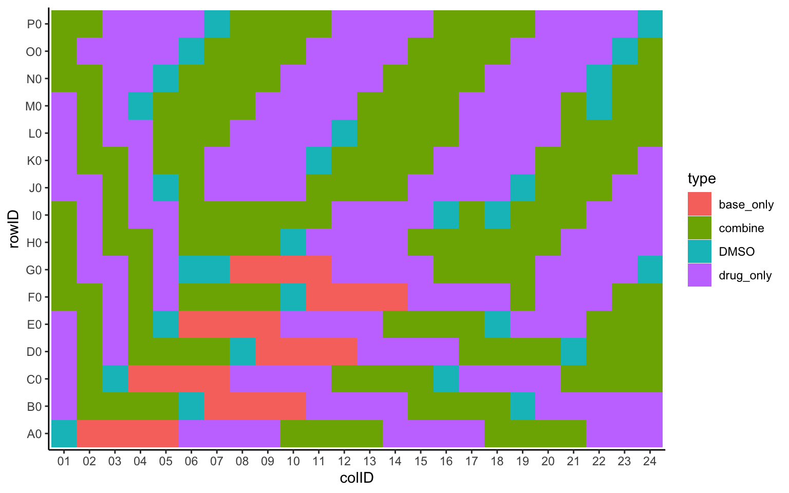
Plot Base drug layout
ggplot(plateLayout, aes(x=colID, y=rowID, fill = Drug_A)) +
    geom_tile() +
    theme_classic()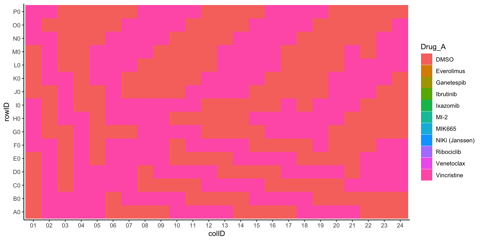
Plot combi drug layout
ggplot(plateLayout, aes(x=colID, y=rowID, fill = Drug_B)) +
    geom_tile() +
theme_classic() 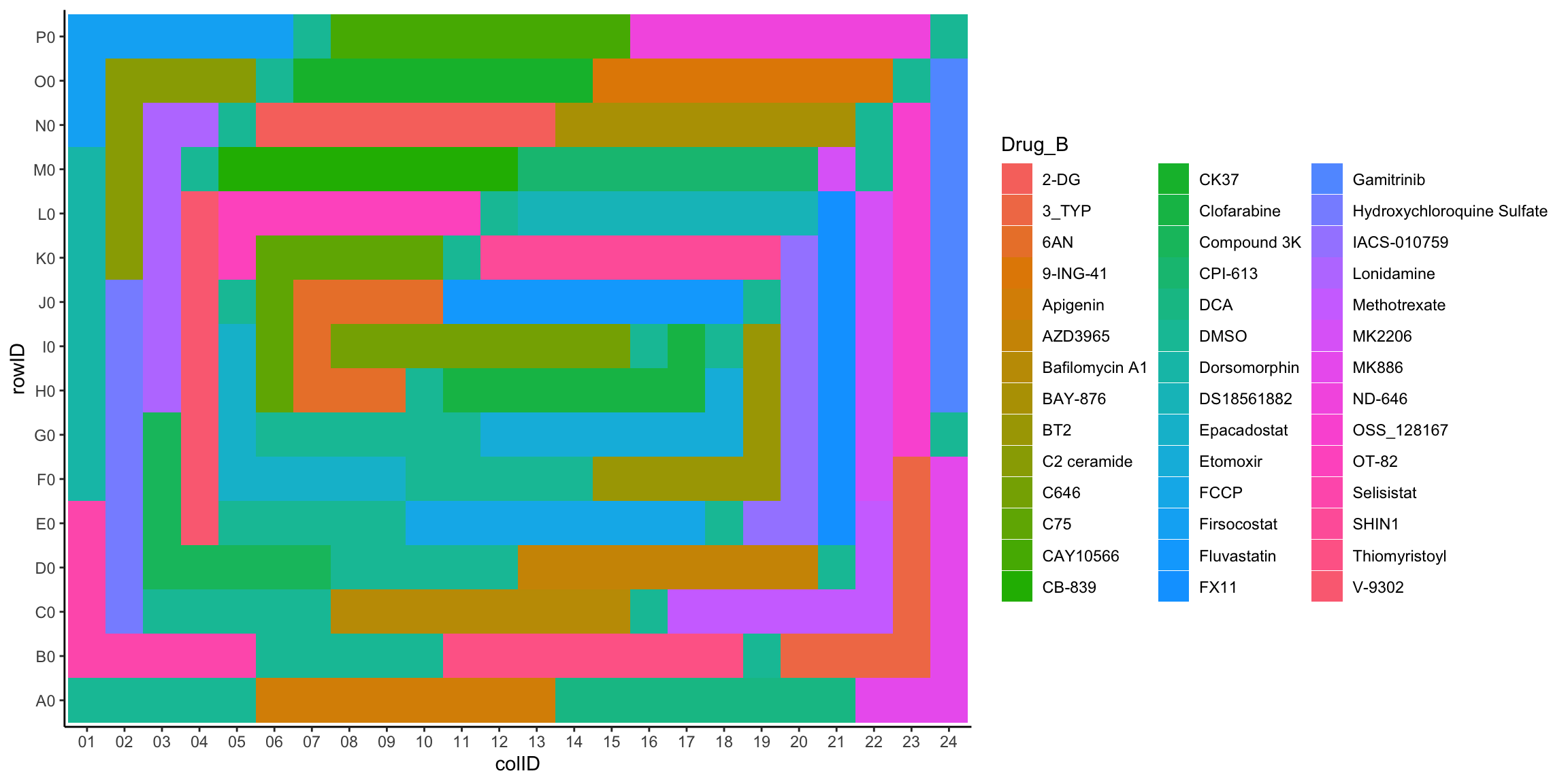
Plot base drug concentration layout
ggplot(plateLayout, aes(x=colID, y=rowID, fill = Drug_A.ConcStep)) +
    geom_tile() +
theme_classic() 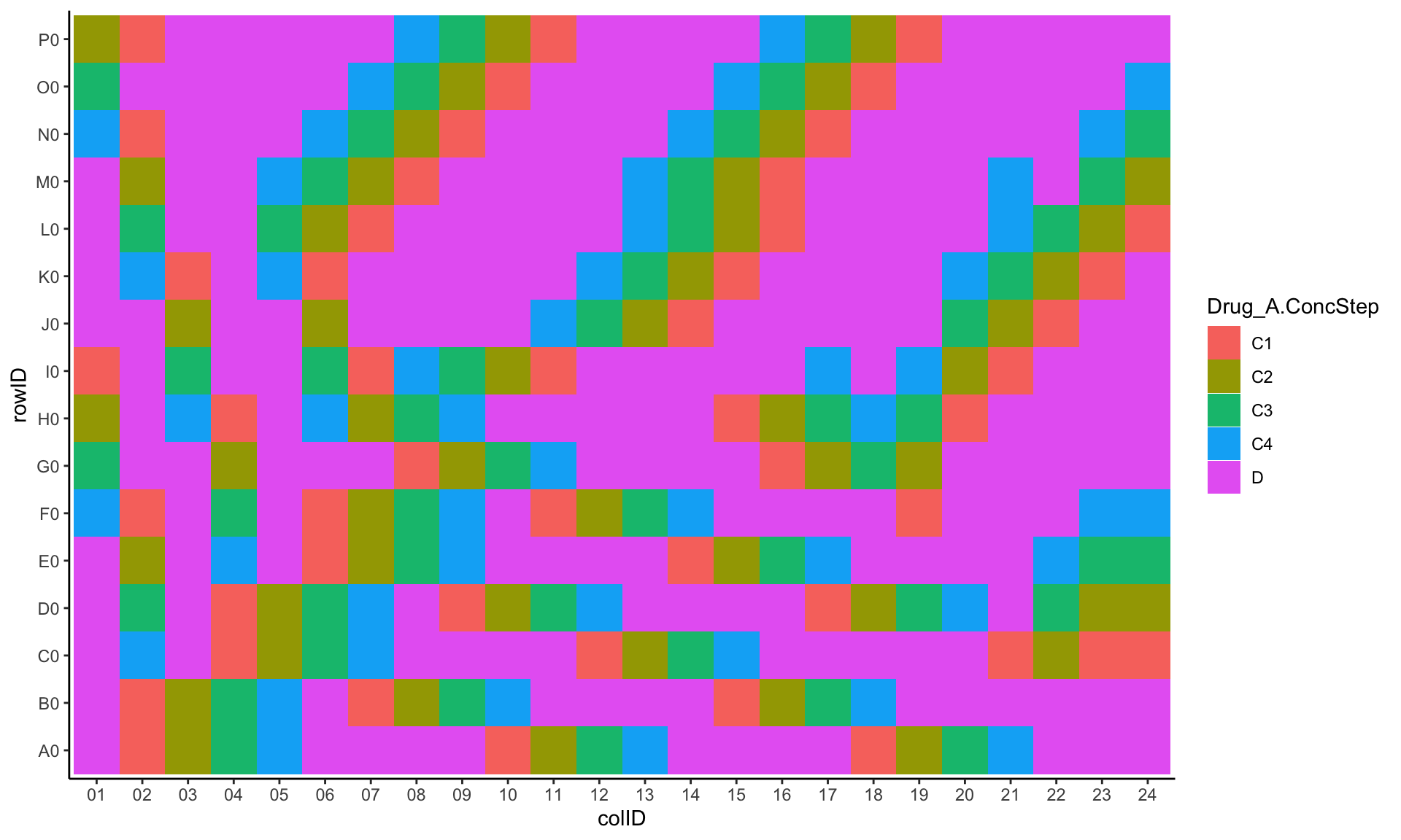
Plot combi drug concentration layour
ggplot(plateLayout, aes(x=colID, y=rowID, fill = Drug_B.ConcStep)) +
    geom_tile() +
theme_classic() 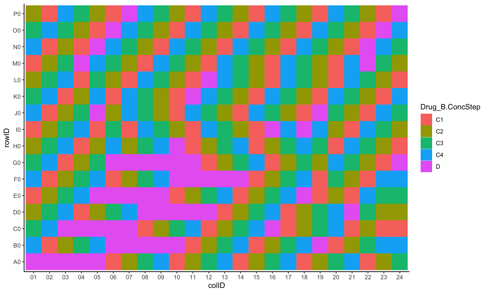
Viability plate plot
pList <- lapply(unique(screenData$plateID), function(id){
    plotTab <- filter(screenData, plateID == id)
    ggplot(plotTab, aes(x=colID, y=rowID, fill = normVal)) +
        geom_tile() +
        scale_fill_gradient2(low = "blue", high = "red", mid = "white", midpoint = 1,limits=c(0,2)) +
        theme_classic() +
        ggtitle(id)
})
jyluMisc::makepdf(pList, "../docs/plate_plot_AA2022.pdf",ncol = 2, nrow = 3, width = 12, height = 12)Check DMSO controls
Mean and Variance of internal controls
plotTab <- filter(screenData, !ifEdge, type == "DMSO")
ggplot(plotTab, aes(x=cellLine, y=value)) +
    ggbeeswarm::geom_quasirandom() +
    theme(axis.text.x = element_text(angle = 90, vjust=0.5, hjust = 1)) +
  facet_wrap(~plate)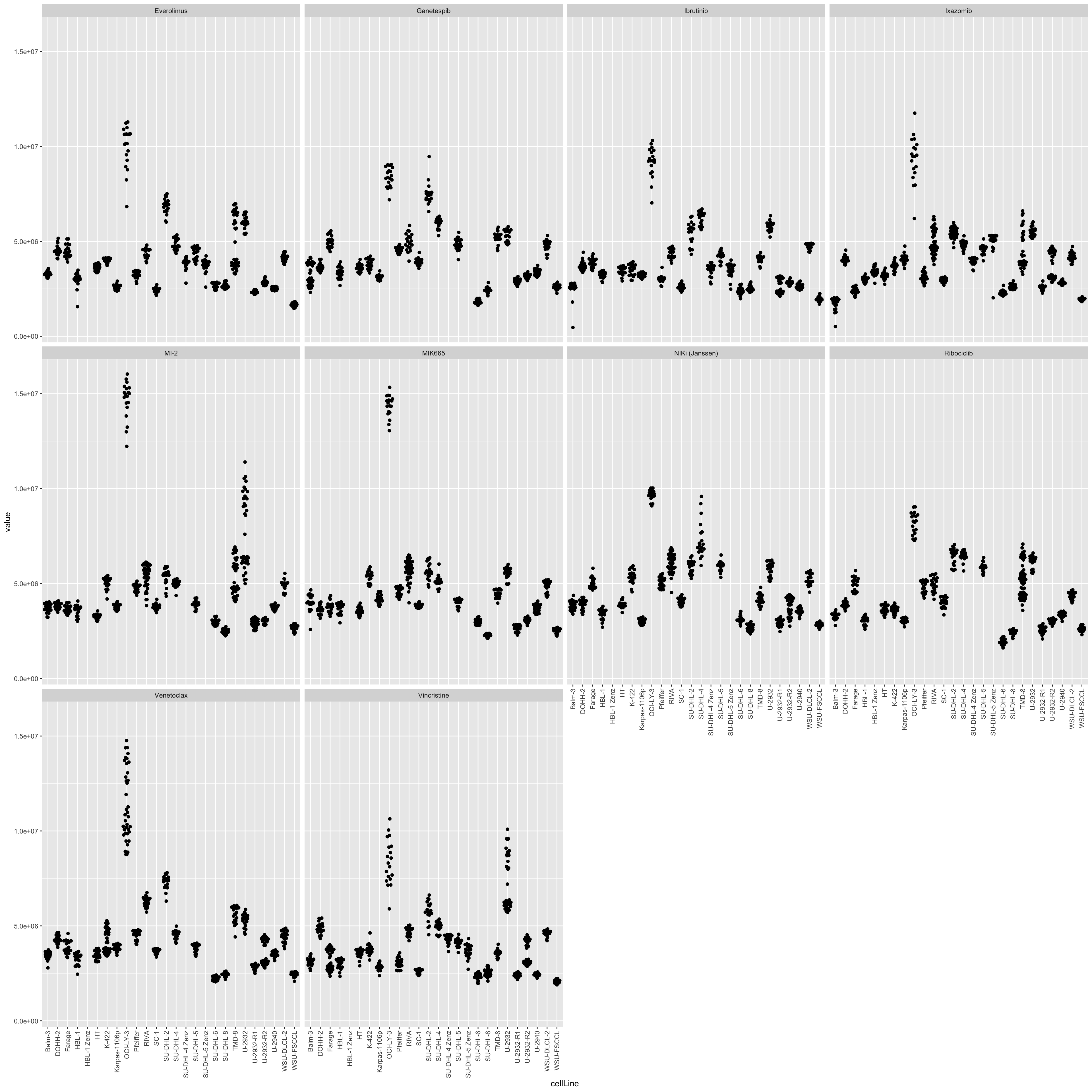
Visualize edge effect
plotTab <- screenData %>% filter(type == "DMSO")
ggplot(plotTab, aes(x=cellLine, y=normVal, col = ifEdge)) +
geom_boxplot() +
theme(axis.text.x = element_text(angle = 90, vjust=0.5, hjust = 1))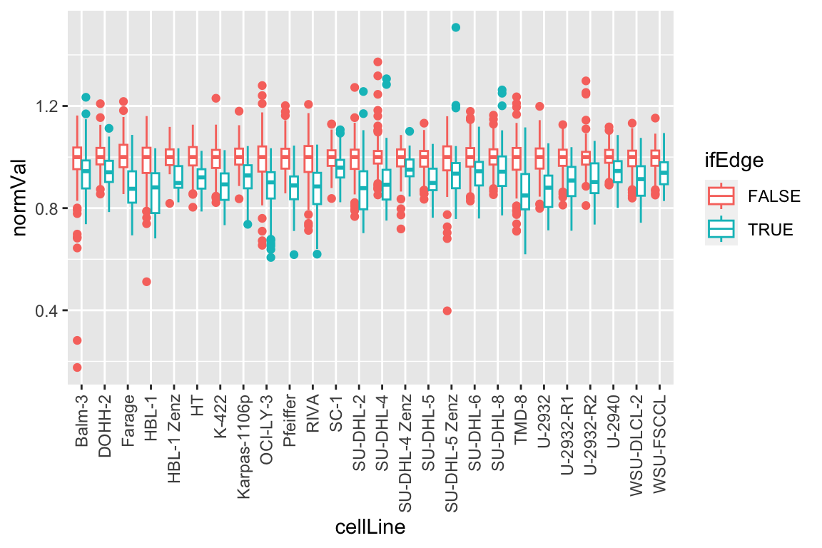 Some degree of edge effect can be observed
Per row
plotTab <- screenData %>% filter(type == "DMSO")
ggplot(plotTab, aes(x=rowID, y=normVal)) +
geom_boxplot() +
theme(axis.text.x = element_text(angle = 90, vjust=0.5, hjust = 1))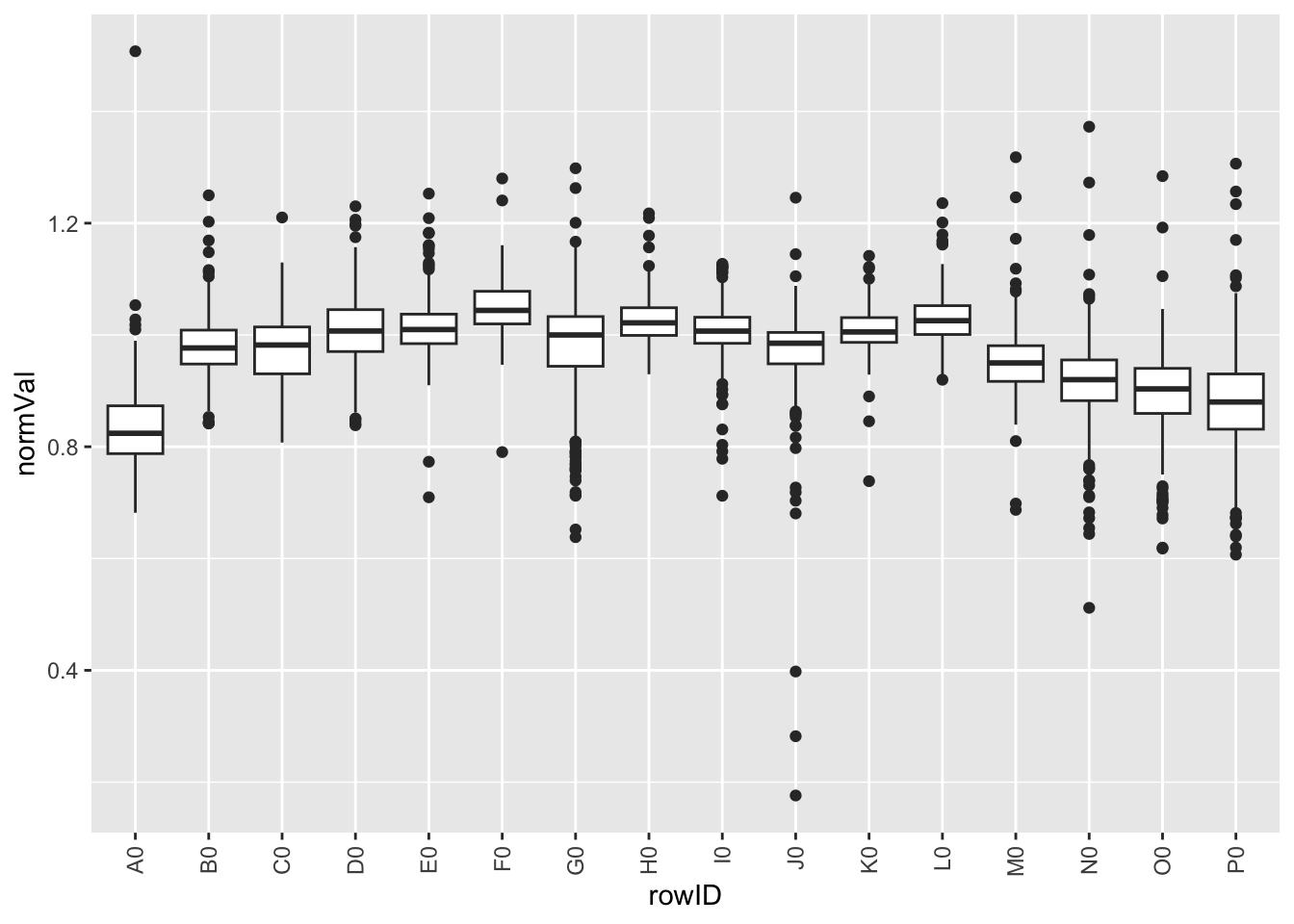 Per column
plotTab <- screenData %>% filter(type == "DMSO")
ggplot(plotTab, aes(x=colID, y=normVal)) +
geom_boxplot() +
theme(axis.text.x = element_text(angle = 90, vjust=0.5, hjust = 1))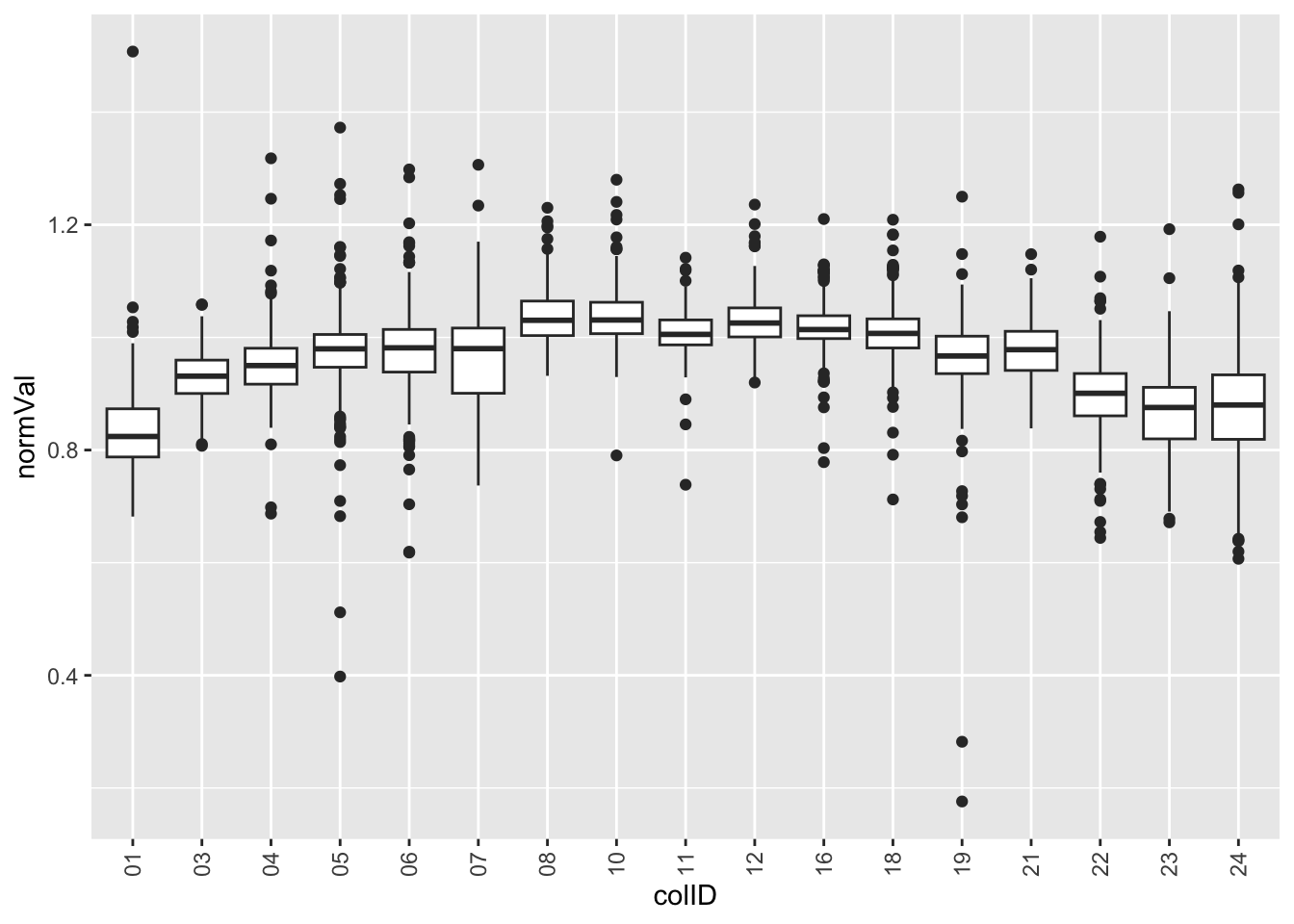 Looks like there’s strong edge effect in this screen.
Correct for edge effect
screenData <- DrugScreenExplorer::correctEdgeEffect(screenData)After correction
plotTab <- screenData %>% filter(type == "DMSO")
ggplot(plotTab, aes(x=cellLine, y=normVal.cor, col = ifEdge)) +
    geom_boxplot() +
    theme(axis.text.x = element_text(angle = 90, vjust=0.5, hjust = 1))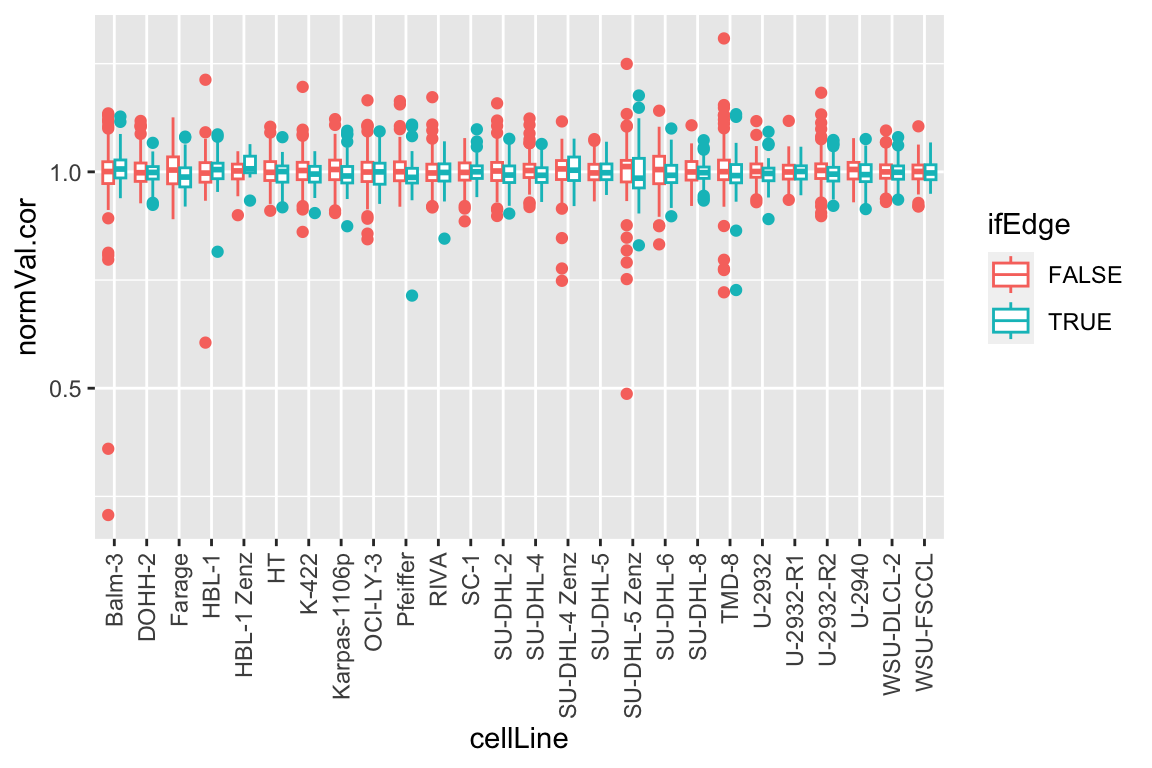
Plate plot after edge correction
pList <- lapply(unique(screenData$plateID), function(id){
    plotTab <- filter(screenData, plateID == id)
    ggplot(plotTab, aes(x=colID, y=rowID, fill = normVal.cor)) +
        geom_tile() +
        scale_fill_gradient2(low = "blue", high = "red", mid = "white", midpoint = 1,limits=c(0,2)) +
        theme_classic() +
        ggtitle(id)
})
jyluMisc::makepdf(pList, "../docs/plate_plot_AA2022_edgeCor.pdf",ncol = 2, nrow = 3, width = 12, height = 12)Visualize Combination design
drugTab <- distinct(screenData, Drug_A, Drug_B, Drug_A.Conc, Drug_B.Conc) %>%
mutate(present = 1) %>%
mutate(drugConcA = paste0(Drug_A,"_",Drug_A.Conc),
drugConcB = paste0(Drug_B, "_", Drug_B.Conc))
countTab <- group_by(screenData, Drug_A, Drug_B, Drug_A.Conc, Drug_B.Conc, cellLine) %>%
summarise(n=length(Drug_A)) %>%
filter(! (Drug_B=="DMSO" & Drug_A == "DMSO"), n>1)
orderA <- arrange(drugTab, Drug_A, Drug_A.Conc)
orderB <- arrange(drugTab, Drug_B, Drug_B.Conc)
designMat <- drugTab %>%
select(drugConcA, drugConcB, present) %>%
pivot_wider(names_from = drugConcB, values_from = present) %>%
pivot_longer(-drugConcA) %>%
mutate(name = factor(name, levels = unique(orderB$drugConcB)),
drugConcA = factor(drugConcA, levels = unique(orderA$drugConcA)))
ggplot(designMat, aes(x=name, y=drugConcA, fill = value)) +
geom_tile() +
theme_minimal() +
theme(axis.text.x = element_text(angle = 90, hjust = 1, vjust=0.5))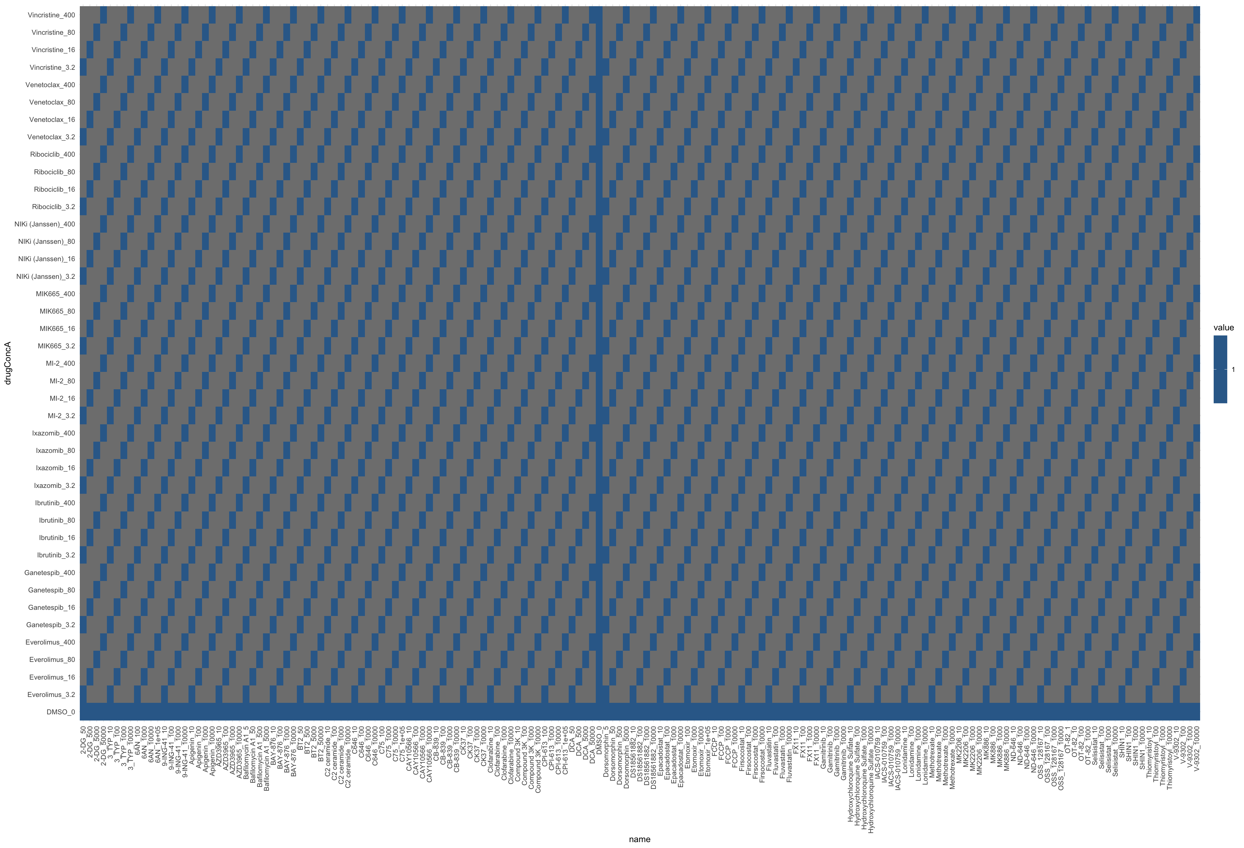 It follows diagonal design.
Visualize single drug effect
Dose response curves of base drugs
drugTab <- distinct(screenData, Drug_A, Drug_B, Drug_B.Conc) %>%
  filter(Drug_A != "DMSO", Drug_B.Conc==0) %>%
  mutate(id = paste0(Drug_A,"_",Drug_B,"_",Drug_B.Conc))

pList.single <- lapply(seq(nrow(drugTab)), function(i) {
  rec <- drugTab[i,]
  plotTab <- filter(screenData,
                    Drug_A == rec$Drug_A,
                    Drug_B == rec$Drug_B,
                    Drug_B.Conc == rec$Drug_B.Conc) %>%
    group_by(Drug_A.Conc, cellLine) %>%
    summarise(normVal = mean(normVal, na.rm=TRUE))

  ggplot(plotTab, aes(x=Drug_A.Conc, y=normVal, group = cellLine, col = cellLine)) +
    geom_line() + geom_point() +
    scale_x_log10() + theme_bw() +
    coord_cartesian(ylim = c(0,1.5)) +
    ggtitle(rec$id) +
    theme(legend.position = "none")
})
names(pList.single) <- drugTab$id

jyluMisc::makepdf(pList.single, "../docs/DoseResponse_base_AA2022.pdf",2,3,width = 8, height = 8)Edge effect corrected
drugTab <- distinct(screenData, Drug_A, Drug_B, Drug_B.Conc) %>%
  filter(Drug_A != "DMSO", Drug_B.Conc==0) %>%
  mutate(id = paste0(Drug_A,"_",Drug_B,"_",Drug_B.Conc))

pList.single <- lapply(seq(nrow(drugTab)), function(i) {
  rec <- drugTab[i,]
  plotTab <- filter(screenData,
                    Drug_A == rec$Drug_A,
                    Drug_B == rec$Drug_B,
                    Drug_B.Conc == rec$Drug_B.Conc) %>%
    group_by(Drug_A.Conc, cellLine) %>%
    summarise(normVal.cor = mean(normVal.cor, na.rm=TRUE))

  ggplot(plotTab, aes(x=Drug_A.Conc, y=normVal.cor, group = cellLine, col = cellLine)) +
    geom_line() + geom_point() +
    scale_x_log10() + theme_bw() +
    coord_cartesian(ylim = c(0,1.5)) +
    ggtitle(rec$id) +
    theme(legend.position = "none")
})
names(pList.single) <- drugTab$id

jyluMisc::makepdf(pList.single, "../docs/DoseResponse_base_AA2022_cor.pdf",2,3,width = 8, height = 8)Dose response curves of combi drugs
drugTab <- distinct(screenData, Drug_A, Drug_B) %>%
  filter(Drug_A == "DMSO", Drug_B!= "DMSO")

pList.combi <- lapply(seq(nrow(drugTab)), function(i) {
  rec <- drugTab[i,]
  plotTab <- filter(screenData,
                    Drug_A == rec$Drug_A,
                    Drug_B == rec$Drug_B) %>%
    group_by(Drug_B.Conc, cellLine) %>%
    summarise(normVal = mean(normVal, na.rm=TRUE))

  ggplot(plotTab, aes(x=Drug_B.Conc, y=normVal, group = cellLine, col = cellLine)) +
    geom_line() + geom_point() +
    scale_x_log10() + theme_bw() +
    coord_cartesian(ylim = c(0,1.5)) +
    ggtitle(paste0(rec$Drug_B)) +
    theme(legend.position = "none")
})
names(pList.combi) <- drugTab$Drug_B

jyluMisc::makepdf(pList.combi, "../docs/DoseResponse_single_AA2022.pdf",2,3,width = 8, height = 8)
DoseResponse_single_AA2022.pdf
Edge effect corrected
drugTab <- distinct(screenData, Drug_A, Drug_B) %>%
  filter(Drug_A == "DMSO", Drug_B!= "DMSO")

pList.combi <- lapply(seq(nrow(drugTab)), function(i) {
  rec <- drugTab[i,]
  plotTab <- filter(screenData,
                    Drug_A == rec$Drug_A,
                    Drug_B == rec$Drug_B) %>%
    group_by(Drug_B.Conc, cellLine) %>%
    summarise(normVal = mean(normVal.cor, na.rm=TRUE))

  ggplot(plotTab, aes(x=Drug_B.Conc, y=normVal, group = cellLine, col = cellLine)) +
    geom_line() + geom_point() +
    scale_x_log10() + theme_bw() +
    coord_cartesian(ylim = c(0,1.5)) +
    ggtitle(paste0(rec$Drug_B)) +
    theme(legend.position = "none")
})
names(pList.combi) <- drugTab$Drug_B

jyluMisc::makepdf(pList.combi, "../docs/DoseResponse_single_AA2022_cor.pdf",2,3,width = 8, height = 8)Check reproducibility in duplicated samples
Find duplicated plates
screenRep <- distinct(screenData, plateID, .keep_all = TRUE) %>%
  arrange(screenDate) %>%
  group_by(plate, cellLine) %>%
  mutate(rep = seq(length(plateID)),
         plateCell = paste0(plate,"_",cellLine)) %>%
  ungroup()

dupPlates <- filter(screenRep, rep >=2) %>%
  distinct(plateCell, plate, cellLine)
dupPlates
# A tibble: 23 × 3
plate cellLine plateCell
<chr> <chr> <chr>
1 Vincristine Farage Vincristine_Farage
2 Venetoclax OCI-LY-3 Venetoclax_OCI-LY-3
3 Ribociclib K-422 Ribociclib_K-422
4 Ganetespib Balm-3 Ganetespib_Balm-3
5 Ribociclib TMD-8 Ribociclib_TMD-8
6 Venetoclax K-422 Venetoclax_K-422
7 Ixazomib SU-DHL-2 Ixazomib_SU-DHL-2
8 Vincristine SU-DHL-8 Vincristine_SU-DHL-8
9 Everolimus TMD-8 Everolimus_TMD-8
10 Ibrutinib U-2932-R1 Ibrutinib_U-2932-R1
# … with 13 more rows
# ℹ Use `print(n = ...)` to see more rowsscreenRep <- filter(screenRep, plateCell %in% dupPlates$plateCell)
#remove the one with three replicates
screenRep <- screenRep %>%
mutate(rep = paste0("R", rep)) %>%
select(plateID, rep, plateCell)Reproducibilities before edge correction
screenSub <- left_join(screenData, screenRep) %>%
  filter(!is.na(rep)) %>%
  select(wellID, normVal, rep, plateCell, type) %>%
  pivot_wider(names_from = rep, values_from = normVal)

ggplot(screenSub, aes(x=R1,y=R2)) +
  geom_point(aes(col=type)) +
  facet_wrap(~plateCell) +
  xlim(0,1.5) + ylim(0,1.5) +
  geom_abline(slope = 1, intercept = 0, color= "red")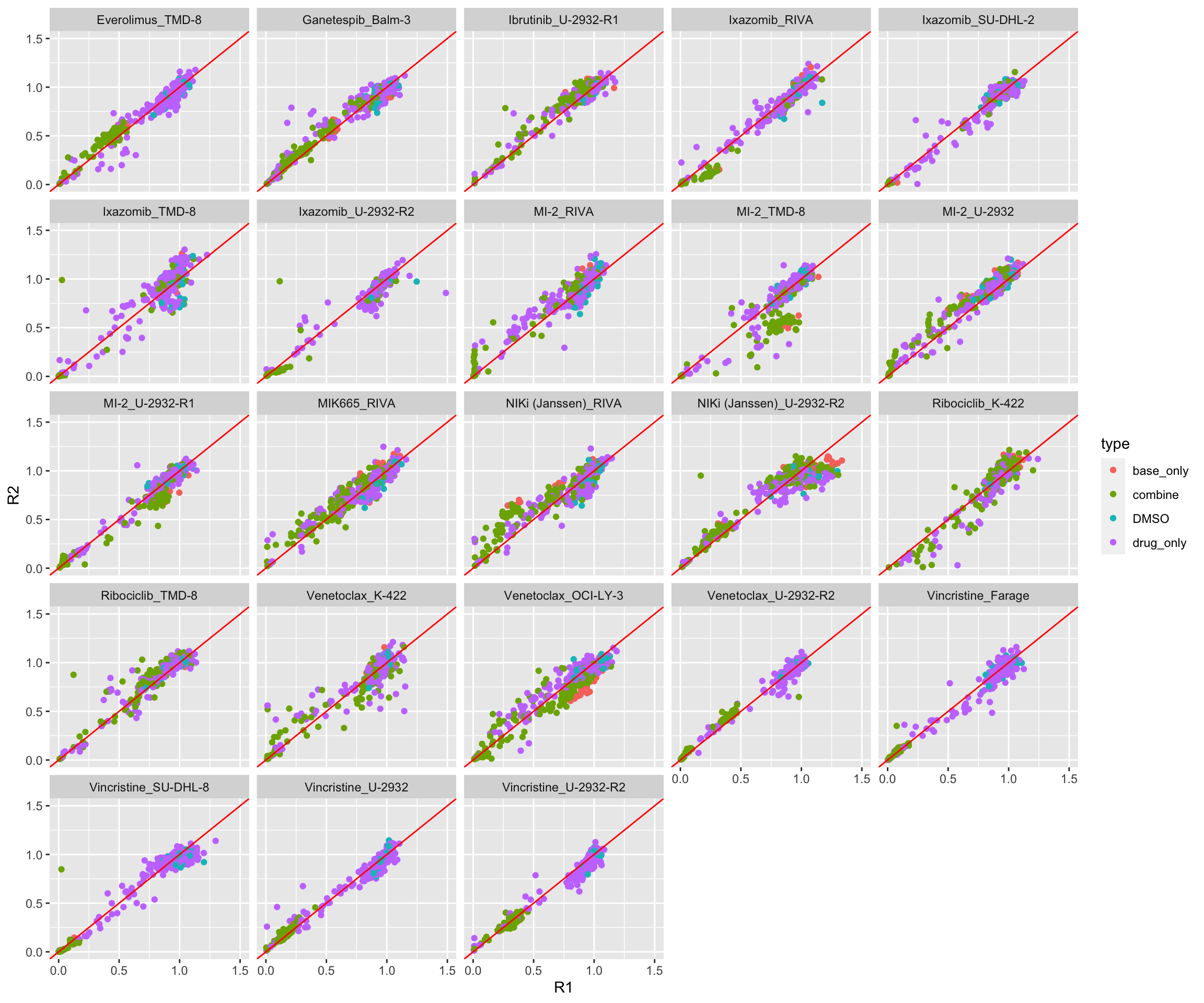
Reproducibilities after edge correction
screenSub <- left_join(screenData, screenRep) %>%
  filter(!is.na(rep)) %>%
  select(wellID, normVal.cor, rep,type, plateCell) %>%
  pivot_wider(names_from = rep, values_from = normVal.cor)

ggplot(screenSub, aes(x=R1,y=R2)) +
  geom_point(aes(col=type)) +
  facet_wrap(~plateCell) +
  xlim(0,1.5) + ylim(0,1.5) +
  geom_abline(slope = 1, intercept = 0, color= "red")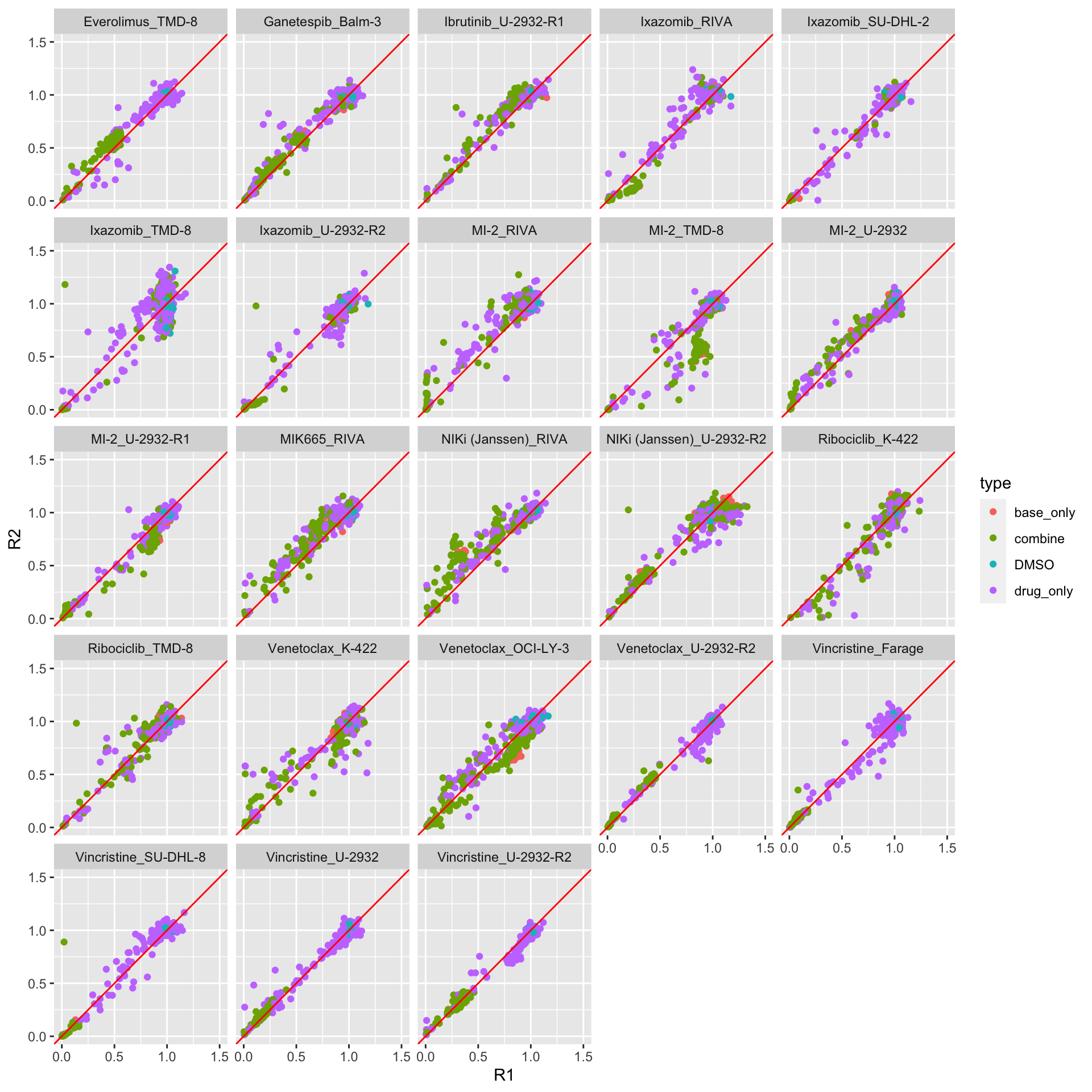
Caclulate R2
screenSub <- left_join(screenData, screenRep) %>%
  filter(!is.na(rep)) %>%
  select(wellID, normVal, normVal.cor, rep, plateCell) %>%
  pivot_longer(c(normVal, normVal.cor), names_to = "correction", values_to = "viability") %>%
  pivot_wider(names_from = rep, values_from = viability)

r2Tab <- group_by(screenSub, plateCell, correction) %>%
  summarise(r2 = cor(R1, R2, use = "pairwise.complete.obs")) %>%
  arrange(mean(r2)) %>%
  mutate(plateCell = factor(plateCell, levels = unique(plateCell)))

ggplot(r2Tab, aes(x= plateCell, y=r2, fill = correction)) +
  geom_bar(stat = "identity", position = "dodge2") +
  theme(axis.text.x = element_text(angle = 90, hjust = 1, vjust = 0.5))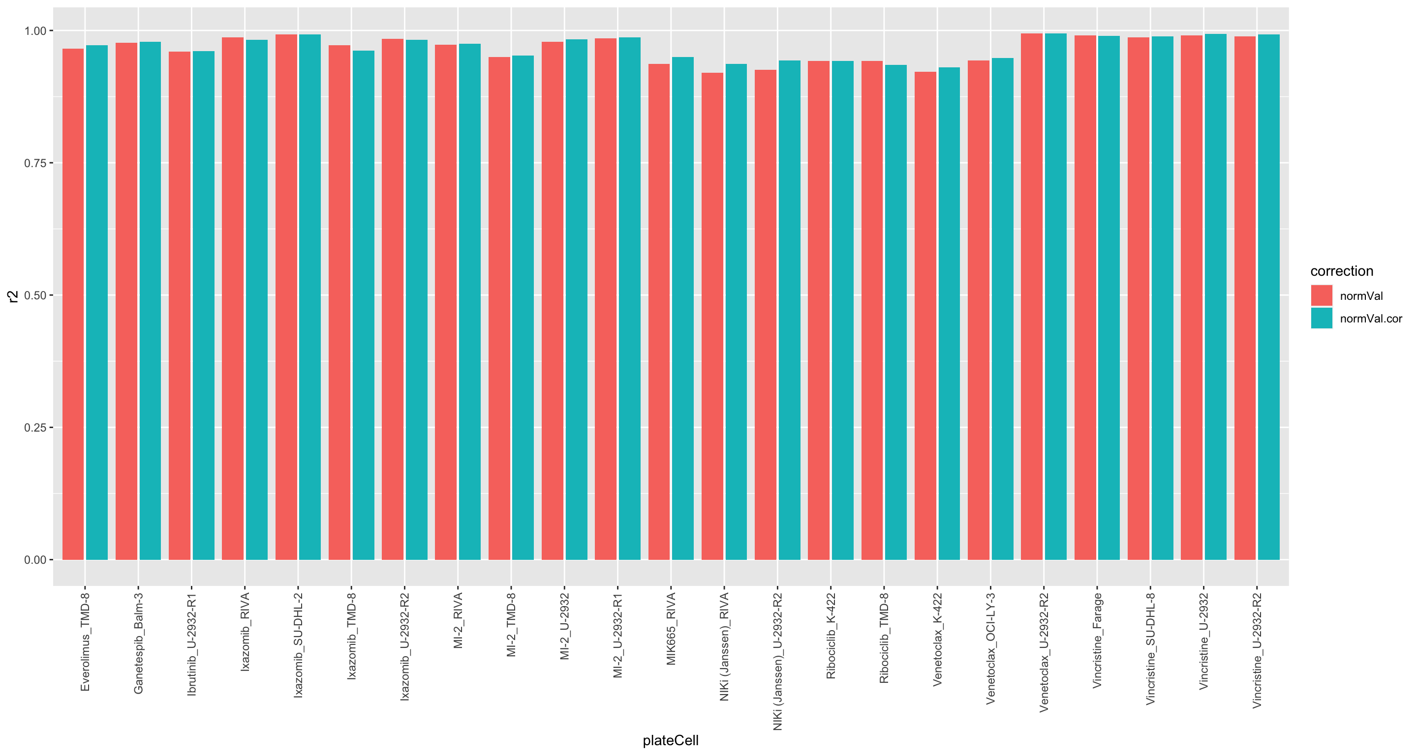
Choose which replicate to use based on the sd of inner DMSO wells
removePlate <- filter(screenData, plateID %in% screenRep$plateID, type == "DMSO", !ifEdge) %>%
  group_by(plateID, plate, cellLine) %>%
  summarise(sd = mad(normVal,na.rm = TRUE)) %>%
  arrange(desc(sd)) %>% ungroup() %>%
  distinct(plate,cellLine, .keep_all = TRUE) %>%
  pull(plateID)

screenData <- mutate(screenData, ifRemove = ifelse(plateID %in% removePlate, TRUE, FALSE))
Save the data object for downstream analyses
#screenData <- mutate(screenData, normVal = normVal.cor)
save(screenData, file = "../output/screenData_AA2022.RData")
save(screenData, file = "../docs/screenData_AA2022.RData")
sessionInfo()R version 4.2.0 (2022-04-22)
Platform: x86_64-apple-darwin17.0 (64-bit)
Running under: macOS Big Sur/Monterey 10.16
Matrix products: default
BLAS: /Library/Frameworks/R.framework/Versions/4.2/Resources/lib/libRblas.0.dylib
LAPACK: /Library/Frameworks/R.framework/Versions/4.2/Resources/lib/libRlapack.dylib
locale:
[1] en_US.UTF-8/en_US.UTF-8/en_US.UTF-8/C/en_US.UTF-8/en_US.UTF-8
attached base packages:
[1] stats graphics grDevices utils datasets methods base
other attached packages:
[1] gridExtra_2.3 forcats_0.5.1 stringr_1.4.1
[4] dplyr_1.0.9 purrr_0.3.4 readr_2.1.2
[7] tidyr_1.2.0 tibble_3.1.8 ggplot2_3.4.1
[10] tidyverse_1.3.2 DrugScreenExplorer_0.1.0
loaded via a namespace (and not attached):
[1] readxl_1.4.0 backports_1.4.1
[3] fastmatch_1.1-3 drc_3.0-1
[5] jyluMisc_0.1.5 workflowr_1.7.0
[7] igraph_1.3.4 shinydashboard_0.7.2
[9] splines_4.2.0 BiocParallel_1.30.3
[11] GenomeInfoDb_1.32.2 TH.data_1.1-1
[13] digest_0.6.30 htmltools_0.5.4
[15] fansi_1.0.3 magrittr_2.0.3
[17] tensor_1.5 googlesheets4_1.0.0
[19] cluster_2.1.3 tzdb_0.3.0
[21] limma_3.52.2 modelr_0.1.8
[23] matrixStats_0.62.0 vroom_1.5.7
[25] sandwich_3.0-2 piano_2.12.0
[27] colorspace_2.0-3 rvest_1.0.2
[29] haven_2.5.0 rbibutils_2.2.9
[31] xfun_0.31 crayon_1.5.2
[33] RCurl_1.98-1.7 jsonlite_1.8.3
[35] survival_3.4-0 zoo_1.8-10
[37] glue_1.6.2 survminer_0.4.9
[39] gtable_0.3.0 gargle_1.2.0
[41] zlibbioc_1.42.0 XVector_0.36.0
[43] DelayedArray_0.22.0 car_3.1-0
[45] BiocGenerics_0.42.0 abind_1.4-5
[47] scales_1.2.0 mvtnorm_1.1-3
[49] DBI_1.1.3 relations_0.6-12
[51] rstatix_0.7.0 Rcpp_1.0.9
[53] plotrix_3.8-2 xtable_1.8-4
[55] bit_4.0.4 km.ci_0.5-6
[57] DT_0.23 stats4_4.2.0
[59] htmlwidgets_1.5.4 httr_1.4.3
[61] fgsea_1.22.0 gplots_3.1.3
[63] ellipsis_0.3.2 pkgconfig_2.0.3
[65] farver_2.1.1 sass_0.4.2
[67] dbplyr_2.2.1 utf8_1.2.2
[69] labeling_0.4.2 tidyselect_1.1.2
[71] rlang_1.0.6 later_1.3.0
[73] visNetwork_2.1.0 munsell_0.5.0
[75] cellranger_1.1.0 tools_4.2.0
[77] cachem_1.0.6 cli_3.4.1
[79] generics_0.1.3 broom_1.0.0
[81] evaluate_0.15 fastmap_1.1.0
[83] yaml_2.3.5 knitr_1.39
[85] bit64_4.0.5 fs_1.5.2
[87] survMisc_0.5.6 caTools_1.18.2
[89] mime_0.12 slam_0.1-50
[91] xml2_1.3.3 compiler_4.2.0
[93] rstudioapi_0.13 beeswarm_0.4.0
[95] ggsignif_0.6.3 marray_1.74.0
[97] reprex_2.0.1 bslib_0.4.1
[99] stringi_1.7.8 highr_0.9
[101] lattice_0.20-45 Matrix_1.4-1
[103] KMsurv_0.1-5 shinyjs_2.1.0
[105] vctrs_0.5.2 pillar_1.8.0
[107] lifecycle_1.0.3 Rdpack_2.4
[109] jquerylib_0.1.4 data.table_1.14.2
[111] cowplot_1.1.1 bitops_1.0-7
[113] httpuv_1.6.6 GenomicRanges_1.48.0
[115] R6_2.5.1 promises_1.2.0.1
[117] KernSmooth_2.23-20 vipor_0.4.5
[119] IRanges_2.30.0 codetools_0.2-18
[121] MASS_7.3-58 gtools_3.9.3
[123] exactRankTests_0.8-35 assertthat_0.2.1
[125] SummarizedExperiment_1.26.1 rprojroot_2.0.3
[127] withr_2.5.0 multcomp_1.4-19
[129] S4Vectors_0.34.0 GenomeInfoDbData_1.2.8
[131] parallel_4.2.0 hms_1.1.1
[133] grid_4.2.0 rmarkdown_2.14
[135] MatrixGenerics_1.8.1 carData_3.0-5
[137] dr4pl_2.0.0 googledrive_2.0.0
[139] ggpubr_0.4.0 git2r_0.30.1
[141] maxstat_0.7-25 sets_1.0-21
[143] Biobase_2.56.0 shiny_1.7.4
[145] lubridate_1.8.0 ggbeeswarm_0.6.0