Introduction

The two instances of modern in the title of this book reflect the two major recent revolutions in biological data analyses:
Biology, formerly a science with sparse, often only qualitative data has turned into a field whose production of quantitative data is on par with high energy physics or astronomy, and whose data are wildly more heterogeneous and complex.
Statistics, a field that in the 20th century had become an application ground for probability theory and calculus, often taught loaded with notation and perceived with a heavy emphasis on hypothesis testing, has been transformed by the ubiquity of computers and of data in machine-readable form. Exploratory data analysis, visualization, resampling, simulations, pragmatic hybridizations of Bayesian ideas and methods with frequentist data analysis have become part of the toolset.
The aim of this book is to enable scientists working in biological research to quickly learn many of the important ideas and methods that they need to make the best of their experiments and of other available data. The book takes a hands-on approach. The narrative is driven by classes of questions, or by certain data types. Methods and theory are introduced on a need-to-know basis. We don’t try to systematically deduce from first principles. The book will often throw readers into the pool and hope they can swim in spite of so many missing details.
By no means this book will replace systematic training in underlying theory: probability, linear algebra, calculus, computer science, databases, multivariate statistics. Such training takes many semesters of coursework. Perhaps the book will whet your appetite to engage more deeply with one of these fields.
The challenge: heterogeneity
Any biological system or organism is composed of tens of thousands of components, which can be in different states and interact in multiple ways. Modern biology aims to understand such systems by acquiring comprehensive –and this means high-dimensional– data in their temporal and spatial context, with multiple covariates and interactions. Dealing with this complexity will be our primary challenge. This includes real, biological complexity as well as the practical complexities and heterogeneities of the data we are able to acquire with our always imperfect instruments.
Biological data come in all sorts of shapes: nucleic acid and protein sequences, rectangular tables of counts, multiple tables, continuous variables, batch factors, phenotypic images, spatial coordinates. Besides data measured in lab experiments, there are clinical data, environmental observations, measurements in space and time, networks and lineage trees, and heaps of previously accumulated knowledge in biological databases as free text or controlled vocabularies, \(...\)
“Homogeneous data are all alike; all heterogeneous data are heterogeneous in their own way.” The Anna Karenina principle.
It is such heterogeneity that motivates our choice of R and Bioconductor as the computational platform for this book – some more on this below.
What’s in this book?
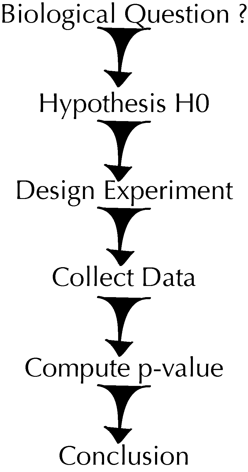
Figure 1 outlines a sequential view of statistical data analysis. Motivated by the groundbreaking work on significance and hypothesis testing in the 1930s by Fisher (1935) and Neyman and Pearson (1936), it is well amenable to mathematical formalism, especially the part where we compute the distribution of test statistics under a hypothesis (null or alternative), or where we need to set up distributional assumptions and can search for analytical approximations.
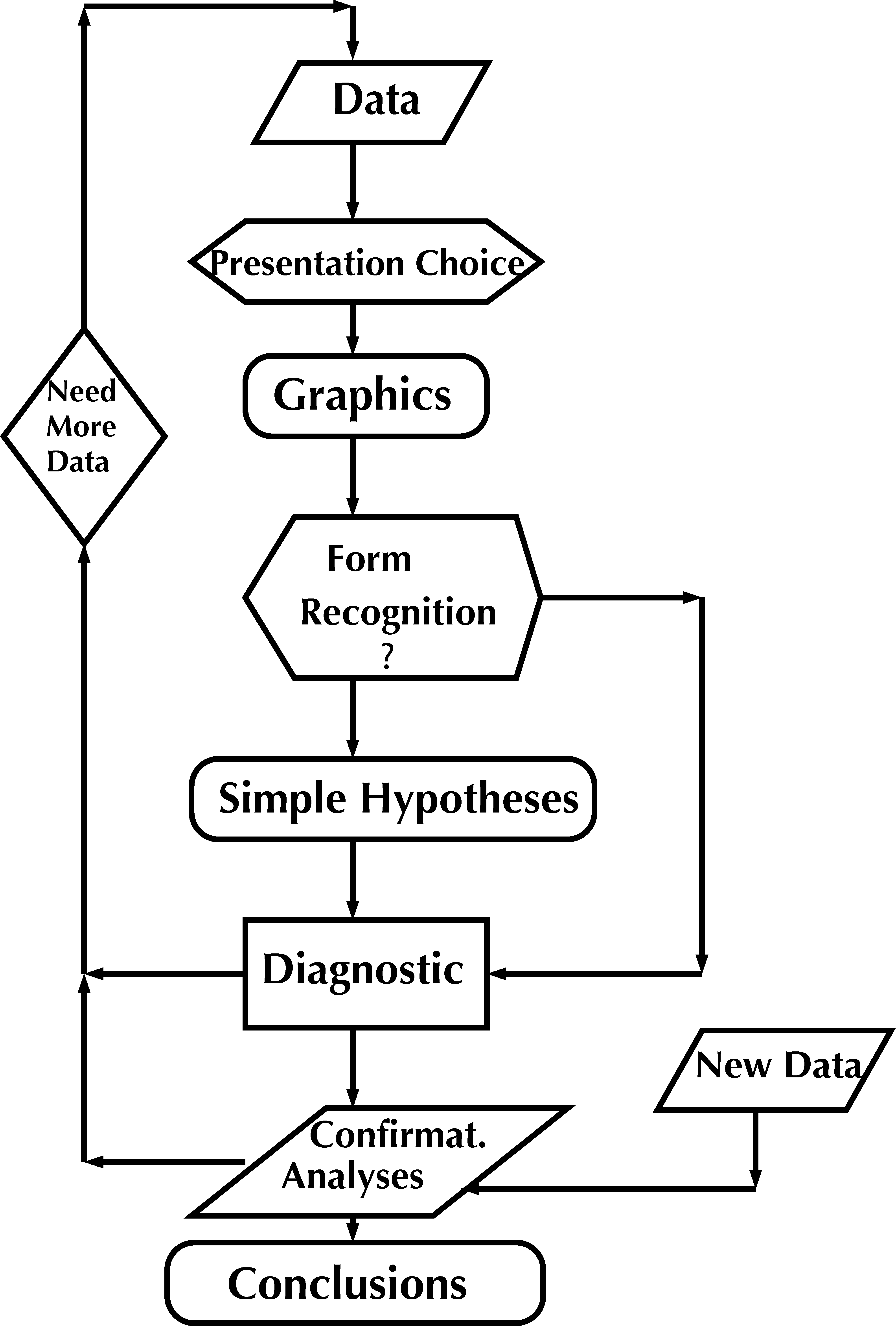
Real scientific discovery rarely works in the caricature manner of Figure 1. Tukey (1977) emphasized two separate approaches. The first he termed exploratory data analysis (EDA). EDA uses the data themselves to decide how to conduct the statistical analysis. EDA is built on data visualization, and then complemented by confirmatory data analyses (CDA): hypothesis-driven inferential methods, which ideally should be robust and not rely on complex assumptions. Tukey recommended an iterative approach schematized in Figure 2 that enable us to see the data at different resolutions and from different perspectives. This enables successive refinement of our understanding of the data and the underlying natural phenomena.
Biology in the late 1990s raised the large-\(p\), small-\(n\) problem: consider a gene expression dataset for \(n=200\) patient-derived tissue samples on \(p=20000\) genes. If we want to construct a regression or classification model that “predicts” a clinical variable, for instance the disease type or outcome, from the \(20000\) genes, or features, we immediately run into problems, since the potential number of model parameters could be orders of magnitudes larger than the number of measurements. The problems derive from non-identifiability of the parameters or overfitting. At least, this is the case for common models, say, an ordinary multivariate linear model. Statisticians realized that they could remedy the situation by requiring sparsity through the use of regularization techniques (Hastie et al. 2008), i.e., by requiring that many of the potential parameters are either zero or at least close to it.
A generalization of the sparsity principle is attained by invoking one of the most powerful recent ideas in high-dimensional statistics, which goes under the name of empirical Bayes: we don’t try to learn all the parameters from scratch, but rather use the fact that groups of them will be similar, or even the same. There are several important book long treatments (Efron 2010) of the subject of large scale inference so essential in modern estimation and hypotheses testing. In the 2010s, computer scientists also discovered ways of engineering “deep neural networks” that can provide sometimes amazing predictive qualities without worrying too much about parameter identifiability or uniqueness.
Simulations play an essential role in this book, as many of the results we need escape the reach of standard analytic approaches. In other words, simulations liberate us from being able to only consider methods that are tractable by “paper and pencil mathematics”, and from worrying about the appropriateness of simplifying assumptions or approximations.
In this book, we try to cover a wide spectrum of these developments and their applications to current biological research. We cover many different types of data that modern biologists have to deal with, including RNA-Seq, flow-cytometry, taxa abundances, imaging data and single cell measurements. We assume no prior formal training in statistics. However, you’ll need some familiarity with R and willingness to engage in mathematical and analytical thinking.

As outlined in the following, the chapters in the book build upon each other, but they are reasonably self-contained, so they can also be studied separately. Each chapter starts with a motivations and goals section. Questions in the text will help you check whether you are following along. The text contains complete R code examples throughout. You don’t need to scrape R code from the HTML or manually copy it from the book. Please use the R files (extension .R) on this website. Each chapter concludes with a summary of the main points and a set of exercises.
Generative models are our basic building blocks. In order to draw conclusions about complicated data it tends to be useful to have simple models for the data generated under this or that situation. We do this through the use of probability theory and generative models, which we introduce in 1 Generative Models for Discrete Data. We will use examples from immunology and DNA analysis to describe useful generative models for biological data: binomial, multinomial and Poisson random variables.
Once we know how data would look like under a certain model, we can start working our way backwards: given some data, what model is most likely able to explain it? This bottom up approach is the core of statistical thinking, and we explain it in 2 Statistical Modeling.
We saw the primary role of graphics in Tukey’s scheme (Figure 2), and so we’ll learn how to visualize our data in 3 Data visualization. We’ll use the grammar of graphics and ggplot2.
Real biological data often have more complex distributional properties than what we could cover in 1 Generative Models for Discrete Data. We’ll use mixtures, which we explore in 4 Mixture Models; these enable us to build realistic models for heterogeneous biological data and provide solid foundations for choosing appropriate variance stabilizing transformations.
The large, matrix-like datasets in biology naturally lend themselves to clustering: once we define a distance measure between matrix rows (the features), we can cluster and group the genes by similarity of their expression patterns, and similarly, for the columns (the patient samples). We’ll cover clustering in 5 Clustering. Since clustering only relies on distances, we can even apply it to data that are not matrix-shaped, as long as there are objects and distances defined between them.
Further following the path of EDA, we cover the most fundamental unsupervised analysis method for simple matrices –principal component analysis– in 7 Multivariate Analysis. We turn to more heterogeneous data that combine multiple data types in 9 Multivariate methods for heterogeneous data. There, we’ll see nonlinear unsupervised methods for counts from single cell data. We’ll also address how to use generalizations of the multivariate approaches covered in 7 Multivariate Analysis to combinations of categorical variables and multiple assays recorded on the same observational units.
The basic hypothesis testing workflow outlined in Figure 1 is explained in 6 Testing. We use the opportunity to apply it to one of the most common queries to \(n\times p\)-datasets: which of the genes (features) are associated with a certain property of the samples, say, disease type or outcome? However, conventional significance thresholds would lead to lots of spurious associations: with a false positive rate of \(\alpha=0.05\) we expect \(p\alpha=1000\) false positives if none of the \(p=20000\) features has a true association. Therefore we also need to deal with multiple testing.
One of the most fruitful ideas in statistics is that of variance decomposition, or analysis of variance (ANOVA). We’ll explore this, in the framework of linear models and generalized linear models, in 8 High-Throughput Count Data & Generalized Linear Models. Since we’ll draw our example data from an RNA-Seq experiment, this gives us also an opportunity to discuss models for such count data, and concepts of robustness.
Nothing in biology makes sense except in the light of evolution1, and evolutionary relationships are usefully encoded in phylogenetic trees. We’ll explore networks and trees in 10 Networks and Trees.
1 Theodosius Dobzhansky, https://en.wikipedia.org/wiki/Nothing_in_Biology_Makes_Sense_Except_in_the_Light_of_Evolution
A rich source of data in biology is images, and in 11 Image data we reinforce our willingness to do EDA on all sorts of heterogeneous data types by exploring feature extraction from images and spatial statistics.
In 12 Supervised Learning, we look at supervised learning: train an algorithm to distinguish between different classes of objects, given a multivariate set of features for each object. We’ll start simple with low-dimensional feature vectors and linear methods, and then step forward to some of the issues of classification in high-dimensional settings. Here, we focus on ‘’classical’’ supervised learning, where (at least conceptually) a training set of ground truth classifications is available to the algorithm all at once, simultaneously, to learn from. We do not (yet…) cover reinforcement learning, a more flexible framework in which one or several agents learn by interacting with a so-called environment by successively performing actions and getting feedback on them; so there are notions of time and state in that framework.
We wrap up in 13 Design of High Throughput Experiments and their Analyses with considerations on good practices in the design of experiments and of data analyses. For this we’ll use and reflect what we have learned in the course of the preceding chapters.
Computational tools for modern biologists
As we’ll see over and over again, the analysis approaches, tools and choices to be made are manifold. Our work can only be validated by keeping careful records in a reproducible script format. R and Bioconductor provide such a platform.
Although we are tackling many different types of data, questions and statistical methods hands-on, we maintain a consistent computational approach by keeping all the computation under one roof: the R programming language and statistical environment, enhanced by the biological data infrastructure and specialized method packages from the Bioconductor project. The reader will have to start by acquiring some familiarity with R before using the book. There are many good books and online resources. One of them is by Grolemund and Wickham (2017), online at http://r4ds.had.co.nz.
R code is a major component of this book. It is how we make the textual explanations explicit. Essentially every data visualization in the book is produced with code that is shown, and the reader should be able to replicate all of these figures, and any other result shown.
Even if you have a some familiarity with R, don’t worry if you don’t immediately understand every line of code in the book. Although we have tried to keep the code explicit and give tips and hints at potentially challenging places, there will be instances where
there is a function invoked that you have not seen before and that does something mysterious,
there is a complicated R expression that you don’t understand (perhaps involving
apply-functions or data manipulations from the dplyr package).
Don’t panic. For the mysterious function, have a look at its manual page. Open up RStudio and use the object explorer to look at the variables that go into the expression, and those that come out. Split up the expression to look at intermediate values.
In Chapters 1 Generative Models for Discrete Data and 2 Statistical Modeling, we use base R functionality for light doses of plotting and data manipulation. As we successively need more sophisticated operations, we introduce the ggplot2 way of making graphics in 3 Data visualization. Besides the powerful grammar of graphics concepts that enable us to produce sophisticated plots using only a limited set of instructions, this implies using the dplyr way of data manipulation.
Why R and Bioconductor?
There are many reasons why we have chosen to present all analyses on the R (Ihaka and Gentleman 1996) and Bioconductor (Huber et al. 2015) platforms:
Cutting edge solutions. The availability of over 20,000 packages ensures that almost all statistical methods are available, including the most recent developments. Moreover, there are implementations of or interfaces to many methods from computer science, mathematics, machine learning, data management, visualization and internet technologies. This puts thousands of person-years of work by experts at your finger tips.
Open source and community-owned. R and Bioconductor have been built collaboratively by a large community of developers. They are constantly tried and tested by thousands of users.
Data input and wrangling. Bioconductor packages support the reading of many of the data types and formats produced by measurement instruments used in modern biology, as well as the needed technology-specific “preprocessing” routines. The community is actively keeping these up-to-date with the rapid developments on the instrument market.
Simulation. There are random number generators for every known statistical distribution and powerful numeric routines for linear algebra, optimization, etc.
Visualization and presentation. R can make attractive, publication-quality graphics. We’ve dedicated 3 Data visualization to this and practice data visualization extensively throughout the book.
Easy to use interactive development environment. RStudio is easy and fun to use and helps with all aspects of programming in R. It is an essential piece in following the iterative approach to data analysis schematized in Figure 2.
Reproducibility. As an equivalent to the laboratory notebook that is standard good practice in labwork, we advocate the use of a computational diary written in the R markdown or quarto formats. We use the quarto system to convert these files into easy-to-read and shareable HTML or PDF documents. These can even become full-fledged scientific articles or supplements. Together with a version control system, this approach also helps with tracking changes.
Collaborative environment. Quarto enables the creation of websites containing code, text, figures and tables with a minimum of work.
Rich data structures. The Bioconductor project has defined specialized data containers to represent complex biological datasets. These help to keep your data consistent, safe and easy to use.
Interoperability and distributed development. Bioconductor in particular contains packages from diverse authors that cover a wide range of functionalities but still interoperate because of the common data containers.
Documentation. Many R packages come with excellent documentation in their function manual pages and vignettes. The vignettes are usually the best starting point into a package, as they give you a high-level narrative on what the package does, whereas the manual pages give detailed information on input, output and inner workings of each function. There are online tutorials, fora and mailing lists for many aspects of working with R and Bioconductor.
High-level language. R is an interpreted high-level language. Its roots in LISP and its functional programming features mean that code is data and can be computed on, which enables efficient programming and is fun. These features facilitate constructing powerful domain specific languages2. R is not a fixed language – throughout its history, it has been actively evolving and is constantly improving.
Page built at 21:13 on 2026-07-15 using R version 4.6.0 (2026-04-24)