2  Statistical Modeling

In the previous chapter, the knowledge of both the generative model and the values of the parameters provided us with probabilities we could use for decision making – for instance, whether we had really found an epitope. In many real situations, neither the generative model nor the parameters are known, and we will need to estimate them using the data we have collected. Statistical modeling works from the data upwards to a model that might plausibly explain the data¹. This upward-reasoning step is called statistical inference. This chapter will show us some of the distributions and estimation mechanisms that serve as building blocks for inference. Although the examples in this chapter are all parametric (i.e., the statistical models only have a small number of unknown parameters), the principles we discuss will generalize.

¹ Even if we have found a model that perfectly explains all our current data, it could always be that reality is more complex. A new set of data lets us conclude that another model is needed, and may include the current model as a special case or approximation.

In a statistical setting, we start with the data \(X\) and use them to estimate the parameters. These estimates are denoted by Greek letters with what we call hats on them, as in \(\widehat{\theta}\).

2.1 Goals for this chapter

In this chapter we will:

• See that there is a difference between two subjects that are often confused: “Probability” and “Statistics”.

• Fit data to probability distributions using histograms and other visualization tricks.

• Have a first encounter with an estimating procedure known as maximum likelihood through a simulation experiment.

• Make inferences from data for which we have prior information. For this we will use the Bayesian paradigm which will involve new distributions with specially tailored properties. We will use simulations and see how Bayesian estimation differs from simple application of maximum likelihood.

• Use statistical models and estimation to evaluate dependencies in binomial and multinomial distributions.

• Analyse some historically interesting genomic data assembled into tables.

• Make Markov chain models for dependent data.

• Do a few concrete applications counting motifs in whole genomes and manipulate special Bioconductor classes dedicated to genomic data.

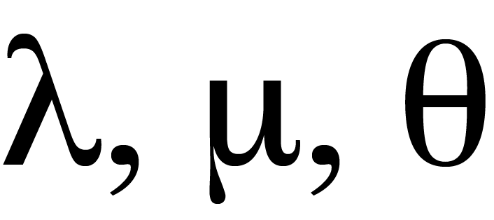
Examples of parameters: the single parameter \(\lambda\) defines a Poisson distribution. The letter \(\mu\) is often used for the mean of the normal. More generally, we use the Greek letter \(\theta\) to designate a generic tuple of parameters necessary to specify a probability model. For instance, in the case of the binomial distribution, \(\theta=(n,p)\) comprises two numbers, a positive integer and a real number between 0 and 1.

Parameters are the key.

We saw in Chapter 1 that the knowledge of all the parameter values in the epitope example enabled us to use our probability model and test a null hypothesis based on the data we had at hand. We will see different approaches to statistical modeling through some real examples and computer simulations, but let’s start by making a distinction between two situations depending on how much information is available.

2.2 The difference between statistical and probabilistic models

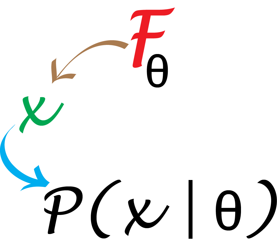
A probabilistic analysis is possible when we know a good generative model for the randomness in the data, and we know its parameters’ actual values.

Figure 2.1: The probabilistic model we obtained in Chapter 1. The data are represented as \(x\) in green. If we know the true value of \(\theta\), then we can compute the probability of observing \(x\) for all possible instances of \(x\), in particular, for an \(x\) that we observed.

In the epitope example, knowing that false positives occur as Bernoulli(0.01) per position, the number of patient samples assayed and the length of the protein, meant that there were no unknown parameters.

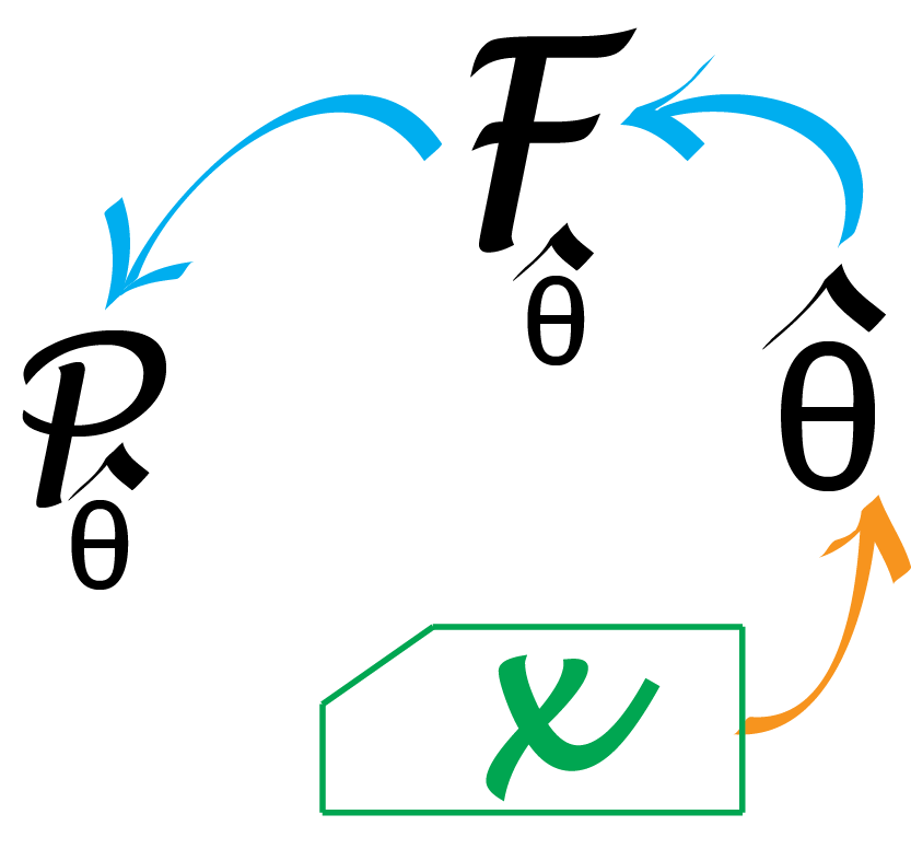
In such a case, we can use mathematical deduction to compute the probability of an event as schematized in Figure 2.1. In the epitope examples, we used the Poisson probability as our null model with the given parameter \(\lambda=0.5\). We were able to conclude through mathematical deduction that the chances of seeing a maximum value of 7 or larger was around \(10^{-4}\) and thus that in fact the observed data were highly unlikely under that model (or “null hypothesis”).

Now suppose that we know the number of patients and the length of the proteins (these are given by the experimental design) but not the distribution itself and the false positive rate. Once we observe data, we need to go up from the data to estimate both a probability model \(F\) (Poisson, normal, binomial) and eventually the missing parameter(s) for that model. This is the type of statistical inference we will explain in this chapter.

2.3 A simple example of statistical modeling

Start with the data

There are two parts to the modeling procedure. First we need a reasonable probability distribution to model the data generation process. As we saw in Chapter 1, discrete count data may be modeled by simple probability distributions such as binomial, multinomial or Poisson distributions. The normal distribution, or bell shaped curve, is often a good model for continuous measurements. Distributions can also be more complicated mixtures of these elementary ones (more on this in Chapter 4).

Let’s revisit the epitope example from the previous chapter, starting without the tricky outlier.

load("../data/e100.RData")
e99 = e100[-which.max(e100)]

Goodness-of-fit : visual evaluation

Our first step is to find a fit from candidate distributions; this requires consulting graphical and quantitative goodness-of-fit plots. For discrete data, we can plot a barplot of frequencies (for continuous data, we would look at the histogram) as in Figure 2.2.

barplot(table(e99), space = 0.8, col = "chartreuse4")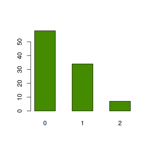

Figure 2.2: The observed distribution of the epitope data without the outlier.

However, it is hard to decide which theoretical distribution fits the data best without using a comparison. One visual goodness-of-fit diagram is known as the rootogram (Cleveland 1988); it hangs the bars with the observed counts from the theoretical red points. If the counts correspond exactly to their theoretical values, the bottom of the boxes will align exactly with the horizontal axis.

library("vcd")
gf1 = goodfit( e99, "poisson")
rootogram(gf1, xlab = "", rect_gp = gpar(fill = "chartreuse4"))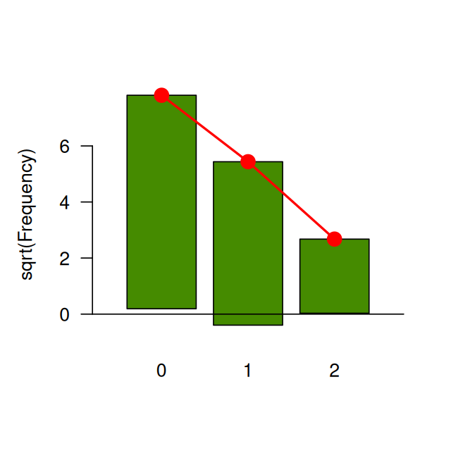

Figure 2.3: Rootogram showing the square root of the theoretical values as red dots and the square root of the observed frequencies as drop down rectangles. (We’ll see a bit below how the goodfit function decided which \(\lambda\) to use.)

Question 2.1

To calibrate what such a plot looks like with a known Poisson variable, use rpois with \(\lambda\) = 0.05 to generate 100 Poisson distributed numbers and draw their rootogram.

Solution

simp = rpois(100, lambda = 0.05)
gf2 = goodfit(simp, "poisson")
rootogram(gf2, xlab = "")

We see that the rootogram for e99 seems to fit the Poisson model reasonably well. But remember, to make this happen we removed the outlier. The Poisson is completely determined by one parameter, often called the Poisson mean \(\lambda\). In most cases where we can guess the data follows a Poisson distribution, we will need to estimate the Poisson parameter from the data.

The parameter is called the Poisson mean because it is the mean of the theoretical distribution and, as it turns out, is estimated by the sample mean. This overloading of the word is confusing to everyone.

The most common way of estimating \(\lambda\) is to choose the value \(\hat{\lambda}\) that makes the observed data the most likely. This is called the maximum likelihood estimator (Rice 2006, chap. 8, Section 5), often abbreviated MLE. We will illustrate this rather paradoxical idea in the next section.

Although we above took out the extreme observation before taking a guess at the probability distribution, we are going to return to the data with it for the rest of our analysis. In practice we would not know whether there is an outlier, and which data point(s) it is / they are. The effect of leaving it in is to make our estimate of the mean higher. In turns this would make it more likely that we’d observe a value of 7 under the null model, resulting in a larger p-value. So, if the resulting p-value is small even with the outlier included, we are assured that our analysis is up to something real. We call such a tactic being conservative: we err on the side of caution, of not detecting something.

Estimating the parameter of the Poisson distribution

What value for the Poisson mean makes the data the most probable? In a first step, we tally the outcomes.

table(e100)

e100
 0  1  2  7 
58 34  7  1 

Then we are going to try out different values for the Poisson mean and see which one gives the best fit to our data. If the mean \(\lambda\) of the Poisson distribution were 3, the counts would look something like this:

table(rpois(100, 3))

 0  1  2  3  4  5  6  7 
 4 13 16 27 21 15  1  3 

which has many more 2’s and 3’s than we see in our data. So we see that \(\lambda=3\) is unlikely to have produced our data, as the counts do not match up so well.

Question 2.2

Repeat this simulation with different values of \(\lambda\). Can you find one that gives counts close to the observed ones just by trial and error?

So we could try out many possible values and proceed by brute force. However, we’ll do something more elegant and use a little mathematics to see which value maximizes the probability of observing our data. Let’s calculate the probability of seeing the data if the value of the Poisson parameter is \(m\). Since we suppose the data derive from independent draws, this probability is simply the product of individual probabilities:

\[\begin{equation*} \begin{aligned} P(58 \times 0, 34 \times 1, 7 \times 2, \text{one }7 \;|\; \text{data are Poisson}(m)) = P(0)^{58}\times P(1)^{34}\times P(2)^{7}\times P(7)^{1}.\end{aligned} \end{equation*}\]

For \(m=3\) we can compute this².

² Note how we here use R’s vectorization: the call to dpois returns four values, corresponding to the four different numbers. We then take these to the powers of 58, 34, 7 and 1, respectively, using the ^ operator, resulting again in four values. Finally, we collapse them into one number, the product, with the prod function.

prod(dpois(c(0, 1, 2, 7), lambda = 3) ^ (c(58, 34, 7, 1)))

[1] 1.392143e-110

Question 2.3

Compute the probability as above for \(m=0,1,2\). Does \(m\) have to be integer? Try computing the probability for \(m=0.4\) for example.

Solution

prod(dpois(c(0, 1, 2, 7), lambda = 0.4) ^ (c(58, 34, 7, 1)))

[1] 8.5483e-46

This probability is the likelihood function of \(\lambda\), given the data, and we write it

Here \(L\) stands for likelihood and \(f(k)=e^{-\lambda} \,\lambda^k\,/\,k!\), the Poisson probability we saw earlier.

\[ L\left(\lambda,\,x=(k_1,k_2,k_3,...)\right)=\prod_{i=1}^{100}f(k_i) \]

Instead of working with multiplications of a hundred small numbers, it is convenient³ to take the logarithm. Since the logarithm is strictly increasing, if there is a point where the logarithm achieves its maximum within an interval it will also be the maximum for the probability.

³ That’s usually true both for pencil and paper and for computer calculations.

⁴ Here we again use R’s vector syntax that allows us to write the computation without an explicit loop over the data points. Compared to the code above, here we call dpois on each of the 100 data points, rather than tabulating data with the table function before calling dpois only on the distinct values. This is a simple example for alternative solutions whose results are equivalent, but may differ in how easy it is to read the code or how long it takes to execute.

Let’s start with a computational illustration. We compute the likelihood for many different values of the Poisson parameter. To do this we need to write a small function that computes the probability of the data for different values⁴.

loglikelihood  =  function(lambda, data = e100) {
  sum(log(dpois(data, lambda)))
}

Now we can compute the likelihood for a whole series of lambda values from 0.05 to 0.95 (Figure 2.4).

lambdas = seq(0.05, 0.95, length = 100)
loglik = vapply(lambdas, loglikelihood, numeric(1))
plot(lambdas, loglik, type = "l", col = "red", ylab = "", lwd = 2,
     xlab = expression(lambda))
m0 = mean(e100)
abline(v = m0, col = "blue", lwd = 2)
abline(h = loglikelihood(m0), col = "purple", lwd = 2)
m0

[1] 0.55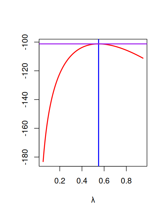

Figure 2.4: The red curve is the log-likelihood function. The vertical line shows the value of m (the mean) and the horizontal line the log-likelihood of m. It looks like m maximizes the likelihood.

Question 2.4

What does the vapply function do in the above code? Hint: check its manual page.

Solution

vapply takes its first argument, the vector lambdas in this case, and iteratively applies the function loglikelihood (its second argument) to each of the vector elements. As a result, it returns a vector of the results. The function also needs a third argument, numeric(1) in this case, that specifies what type of value each individual call to loglikelihood is supposed to return: a single number. (In general, it could happen that the function sometimes returns something else, say, a character string, or two numbers; in that case it would not be possible to assemble the overall results into a coherent vector, and vapply would complain.)

In fact there is a shortcut: the function goodfit.

gf  =  goodfit(e100, "poisson")
names(gf)

[1] "observed" "count"    "fitted"   "type"     "method"   "df"       "par"     

gf$par

$lambda
[1] 0.55

The output of goodfit is a composite object called a list. One of its components is called par and contains the value(s) of the fitted parameter(s) for the distribution studied. In this case it’s only one number, the estimate of \(\lambda\).

Question 2.5

What are the other components of the output from the goodfit function?

Task

Compare the value of m to the value that we used previously for \(\lambda\), 0.5. Redo the modeling that we did in Chapter 1 with m instead of 0.5.

2.3.1 Classical statistics for classical data

Here is a formal proof of our computational finding that the sample mean maximizes the (log-)likelihood.

\[ \begin{align} \log L(\lambda, x) &= \sum_{i=1}^{100} - \lambda + k_i\log\lambda - \log(k_i!) \\ &= -100\lambda + \log\lambda\left(\sum_{i=1}^{100}k_i\right) + \text{const.} \end{align} \tag{2.1}\]

We use the catch-all “const.” for terms that do not depend on \(\lambda\) (although they do depend on \(x\), i.e., on the \(k_i\)). To find the \(\lambda\) that maximizes this, we compute the derivative in \(\lambda\) and set it to zero.

\[ \begin{align} \frac{d}{d\lambda}\log L &= -100 + \frac{1}{\lambda} \sum_{i=1}^{100}k_i \stackrel{?}{=}0 \\ \lambda &= \frac{1}{100} \sum_{i=1}^{100}k_i = \bar{k} \end{align} \tag{2.2}\]

You have just seen the first steps of a statistical approach, starting `from the ground up’ (from the data) to infer the model parameter(s): this is statistical estimation of a parameter from data. Another important component will be choosing which family of distributions we use to model our data; that part is done by evaluating the goodness of fit. We will encounter this later.

In the classical statistical testing framework, we consider one single model, that we call the null model, for the data. The null model formulates an “uninteresting” baseline, such as that all observations come from the same random distribution regardless of which group or treatment they are from. We then test whether there is something more interesting going on by computing the probability that the data are compatible with that model. Often, this is the best we can do, since we do not know in sufficient detail what the “interesting”, non-null or alternative model should be. In other situations, we have two competing models that we can compare, as we will see later.

Question 2.6

What is the value of modeling with a known distribution? For instance, why is it interesting to know a variable has a Poisson distribution ?

Solution

Models are concise but expressive representations of the data generating process. For the Poisson for instance, knowing one number allows us to know everything about the distribution, including, as we saw earlier, the probabilities of extreme or rare events.

Another useful direction is regression. We may be interested in knowing how our count-based response variable (e.g., the result of counting sequencing reads) depends on a continuous covariate, say, temperature or nutrient concentration. You may already have encountered linear regression, where our model is that the response variable \(y\) depends on the covariate \(x\) via the equation \(y = ax+b + e\), with parameters \(a\) and \(b\) (that we need to estimate), and with residuals \(e\) whose probability model is a normal distribution (whose variance we usually also need to estimate). For count data the same type of regression model is possible, although the probability distribution for the residuals then needs to be non-normal. In that case we use the generalized linear models framework. We will see examples when studying RNA-Seq in Chapter 8 and another type of next generation sequencing data, 16S rRNA data, in Chapter 9.

Knowing that our probability model involves a Poisson, binomial, multinomial distribution or another parametric family will enable us to have quick answers to questions about the parameters of the model and compute quantities such as p-values and confidence intervals.

2.4 Binomial distributions and maximum likelihood

In a binomial distribution there are two parameters: the number of trials \(n\), which is typically known, and the probability \(p\) of seeing a 1 in a trial. This probability is often unknown.

2.4.1 An example

Suppose we take a sample of \(n=120\) males and test them for red-green colorblindness. We can code the data as 0 if the subject is not colorblind and 1 if he is. We summarize the data by the table:

table(cb)

cb
  0   1 
110  10 

Question 2.7

Which value of \(p\) is the most likely given these data?

Solution

\(\hat{p}=\frac{1}{12}\).

mean(cb)

[1] 0.08333333

However, be careful: sometimes, maximum likelihood estimates are harder to guess and to compute, as well as being much less intuitive (see Exercise 2.2).

In this special case, your intuition may give you the estimate \(\hat{p}=\frac{1}{12}\), which turns out to be the maximum likelihood estimate. We put a hat over the letter to remind us that this is not (necessarily) the underlying true value, but an estimate we make from the data.

As before in the case of the Poisson, if we compute the likelihood for many possible \(p\), we can plot it and see where its maximum falls (Figure 2.5).

probs  =  seq(0, 0.3, by = 0.005)
likelihood = dbinom(sum(cb), prob = probs, size = length(cb))
plot(probs, likelihood, pch = 16, xlab = "probability of success",
       ylab = "likelihood", cex=0.6)
probs[which.max(likelihood)]

[1] 0.085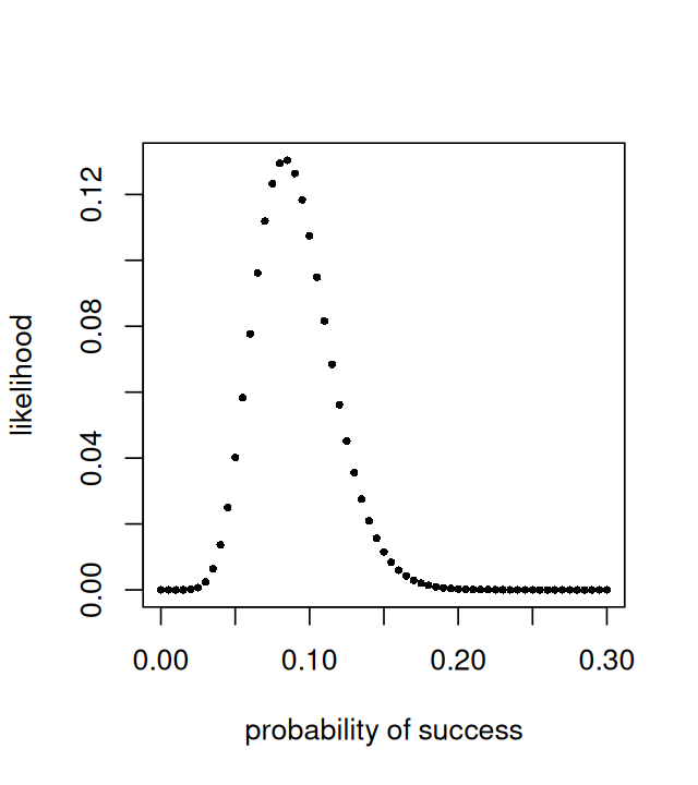

Figure 2.5: Plot of the likelihood as a function of the probabilities. The likelihood is a function on \([0, 1]\). Here we have zoomed into the range of \([0, 0.3]\), as the likelihood is practically zero for larger values of \(p\).

Note: 0.085 is not exactly the value we expected \((\frac{1}{12})\), and that is because the set of values that we tried (in probs) did not include the exact value of \(\frac{1}{12}\simeq 0.0833\), so we obtained the next best one. We could use numeric optimisation methods to overcome that.

2.4.2 Likelihood for the binomial distribution

One can come up with different criteria than maximum likelihood, which lead to other estimators. They all carry hats. We’ll see other examples in Chapter 4.

The likelihood and the probability are the same mathematical function, only interpreted in different ways – in one case, the function tells us how probable it is to see a particular set of values of the data, given the parameters; in the other case, we consider the data as given, and ask for the parameter value(s) that likely generated these data. Suppose \(n=300\), and we observe \(y=40\) successes. Then, for the binomial distribution:

\[ f(p\,|\,n,y) = f(y\,|\,n,p)={n \choose y} \, p^y \, (1-p)^{(n-y)}. \tag{2.3}\]

Again, it is more convenient to work with the logarithm of the likelihood,

\[ \log f(p |y) = \log {n \choose y} + y\log(p) + (n-y)\log(1-p). \tag{2.4}\]

Here’s a function we can use to calculate it⁵,

⁵ In practice, we would try to avoid explicitly computing choose(n, y), since it can be a very large number that tests the limits of our computer’s floating point arithmetic (for n=300 and y=40, it is around 9.8e+49). One could approximate the term using Stirling’s formula, or indeed ignore it, as it is only an additive offset independent of \(p\) that does not impact the maximization.

loglikelihood = function(p, n = 300, y = 40) {
  log(choose(n, y)) + y * log(p) + (n - y) * log(1 - p)
}

which we plot for the range of \(p\) from 0 to 1 (Figure 2.6).

p_seq = seq(0, 1, by = 0.001)
plot(p_seq, loglikelihood(p_seq), xlab = "p", ylab = "log f(p|y)", type = "l")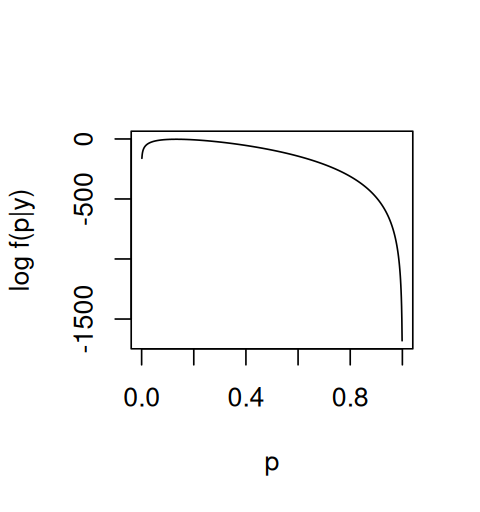

Figure 2.6: Plot of the log likelihood function for \(n=300\) and \(y=40\).

The maximum lies at 40/300 = 0.1333… , consistent with intuition, but we see that other values of \(p\) are almost equally likely, as the function is quite flat around the maximum. We will see in a later section how Bayesian methods enable us to work with a range of values for \(p\) instead of just picking a single maximum.

2.5 More boxes:multinomial data

2.5.1 DNA count modeling: base pairs

There are four basic molecules of DNA: A - adenine, C - cytosine, G - guanine, T - thymine. The nucleotides are classified into 2 groups: purines (A and G) and pyrimidines (C and T). The binomial would work as a model for the purine/pyrimidine groupings but not if we want to use A, C, G, T; for that we need the multinomial model from Section 1.4. Let’s look at noticeable patterns that occur in these frequencies.

2.5.2 Nucleotide bias

This section combines estimation and testing by simulation in a real example. Data from one strand of DNA for the genes of Staphylococcus aureus bacterium are available in a fasta file staphsequence.ffn.txt, which we can read with a function from the Bioconductor package Biostrings.

library("Biostrings")
staph = readDNAStringSet("../data/staphsequence.ffn.txt", "fasta")

Let’s look at the first gene:

staph[1]

DNAStringSet object of length 1:
    width seq                                               names               
[1]  1362 ATGTCGGAAAAAGAAATTTGGGA...AAAAAGAAATAAGAAATGTATAA lcl|NC_002952.2_c...

letterFrequency(staph[[1]], letters = "ACGT", OR = 0)

  A   C   G   T 
522 219 229 392 

Question 2.8

Why did we use double square brackets in the second line?

Solution

The double square brackets [[i]] extract the sequence of the i-th gene as a DNAString, as opposed to the pair of single brackets [i], which return a DNAStringSet with just a single DNAString in it. If you look at the length of staph[1], it is 1, whereas staph[[1]] has length 1362.

Question 2.9

Following a similar procedure as in Exercise 1.8, test whether the nucleotides are equally distributed across the four nucleotides for this first gene.

Due to their different physical properties, evolutionary selection can act on the nucleotide frequencies. So we can ask whether, say, the first ten genes from these data come from the same multinomial. We do not have a prior reference, we just want to decide whether the nucleotides occur in the same proportions in the first 10 genes. If not, this would provide us with evidence for varying selective pressure on these ten genes.

letterFrq = vapply(staph, letterFrequency, FUN.VALUE = numeric(4),
         letters = "ACGT", OR = 0)
colnames(letterFrq) = paste0("gene", seq(along = staph))
tab10 = letterFrq[, 1:10]
computeProportions = function(x) { x/sum(x) }
prop10 = apply(tab10, 2, computeProportions)
round(prop10, digits = 2)

  gene1 gene2 gene3 gene4 gene5 gene6 gene7 gene8 gene9 gene10
A  0.38  0.36  0.35  0.37  0.35  0.33  0.33  0.34  0.38   0.27
C  0.16  0.16  0.13  0.15  0.15  0.15  0.16  0.16  0.14   0.16
G  0.17  0.17  0.23  0.19  0.22  0.22  0.20  0.21  0.20   0.20
T  0.29  0.31  0.30  0.29  0.27  0.30  0.30  0.29  0.28   0.36

p0 = rowMeans(prop10)
p0

        A         C         G         T 
0.3470531 0.1518313 0.2011442 0.2999714 

So let’s suppose p0 is the vector of multinomial probabilities for all the ten genes and use a Monte Carlo simulation to test whether the departures between the observed letter frequencies and expected values under this supposition are within a plausible range.

We compute the expected counts by taking the outer product of the vector of probabilities p0 with the sums of nucleotide counts from each of the 10 columns, cs.

cs = colSums(tab10)
cs

 gene1  gene2  gene3  gene4  gene5  gene6  gene7  gene8  gene9 gene10 
  1362   1134    246   1113   1932   2661    831   1515   1287    696 

expectedtab10 = outer(p0, cs, FUN = "*")
round(expectedtab10)

  gene1 gene2 gene3 gene4 gene5 gene6 gene7 gene8 gene9 gene10
A   473   394    85   386   671   924   288   526   447    242
C   207   172    37   169   293   404   126   230   195    106
G   274   228    49   224   389   535   167   305   259    140
T   409   340    74   334   580   798   249   454   386    209

We can now create a random table with the correct column sums using the rmultinom function. This table is generated according to the null hypothesis that the true proportions are given by p0.

randomtab10 = sapply(cs, function(s) { rmultinom(1, s, p0) } )
all(colSums(randomtab10) == cs)

[1] TRUE

Now we repeat this B = 1000 times. For each table we compute our test statistic from Section 1.4.1 in Chapter 1 (the function stat) and store the results in the vector simulstat. Together, these values constitute our null distribution, as they were generated under the null hypothesis that p0 is the vector of multinomial proportions for each of the 10 genes.

stat = function(obsvd, exptd) {
   sum((obsvd - exptd)^2 / exptd)
}
B = 1000
simulstat = replicate(B, {
  randomtab10 = sapply(cs, function(s) { rmultinom(1, s, p0) })
  stat(randomtab10, expectedtab10)
})
S1 = stat(tab10, expectedtab10)
sum(simulstat >= S1)

[1] 0

hist(simulstat, col = "lavender", breaks = seq(0, 75, length.out=50))
abline(v = S1, col = "red")
abline(v = quantile(simulstat, probs = c(0.95, 0.99)),
       col = c("darkgreen", "blue"), lty = 2)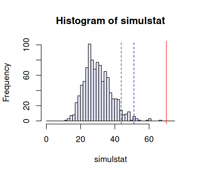

Figure 2.7: Histogram of simulstat. The value of S1 is marked by the vertical red line, those of the 0.95 and 0.99 quantiles (see next section) by the dotted lines.

The histogram is shown in Figure 2.7. We see that the probability of seeing a value as large as S1=70.1 is very small under the null model. It happened 0 times in our 1000 simulations that a value as big as S1 occurred. Thus the ten genes do not seem to come from the same multinomial model.

2.6 The \(\chi^2\) distribution

In fact, we could have used statistical theory to come to the same conclusion without running these simulations. The theoretical distribution of the simulstat statistic is called the \(\chi^2\) (chi-squared) distribution⁶ with parameter 30 (\(=10\times(4-1)\)). We can use this for computing the probability of having a value as large as S1 \(=\) 70.1. As we just saw above, small probabilities are difficult to compute by Monte Carlo: the granularity of the computation is \(1/B\), so we cannot estimate any probabilities smaller than that, and in fact the uncertainty of the estimate is larger. So if any theory is applicable, that tends to be useful. We can check how well theory and simulation match up in our case using another visual goodness-of-fit tool: the quantile-quantile (QQ) plot. When comparing two distributions, whether from two different samples or from one sample versus a theoretical model, just looking at histograms is not informative enough. We use a method based on the quantiles of each of the distributions.

⁶ Strictly speaking, the distribution of simulstat is approximately described by a \(\chi^2\) distribution; the approximation is particularly good if the counts in the table are large.

2.6.1 Intermezzo: quantiles and the quantile-quantile plot

In the previous chapter, we ordered the 100 sample values \(x_{(1)},x_{(2)},...,x_{(100)}\). Say we want the 22nd percentile. We can take any value between the 22nd and the 23rd value, i.e., any value that fulfills \(x_{(22)} \leq c_{0.22} < x_{(23)}\) is acceptable as a 0.22 quantile (\(c_{0.22}\)). In other words, \(c_{0.22}\) is defined by

\[ \frac{\# x_i's \leq c_{0.22}}{n} = 0.22. \]

In Section 3.6.7, we’ll introduce the empirical cumulative distribution function (ECDF) \(\hat{F}\), and we’ll see that our definition of \(c_{0.22}\) can also be written as \(\hat{F}_n(c_{0.22}) = 0.22\). In Figure 2.7, our histogram of the distribution of simulstat, the quantiles \(c_{0.95}\) and \(c_{0.99}\) are also shown.

Question 2.10

1. Compare the simulstat values and 1000 randomly generated \(\chi^2_{30}\) random numbers by displaying them in histograms with 50 bins each.

2. Compute the quantiles of the simulstat values and compare them to those of the \(\chi_{30}^2\) distribution. Hint:

qs = ppoints(100)
quantile(simulstat, qs)
quantile(qchisq(qs, df = 30), qs)

A name collision occurs here. Statisticians call the summary statistic we just computed as simulstat (sum of squares of weighted differences), the chi-squared or \(\chi^2\) statistic. The theoretical distribution \(\chi^2_\nu\) is a distribution in its own right, with a parameter \(\nu\) called the degrees of freedom. When reading about the chi-squared or \(\chi^2\), you will need to pay attention to the context to see which meaning is appropriate.

Question 2.11

Do you know another name for the 0.5 quantile?

Solution

The median.

Question 2.12

In the above definition, we were a little vague on how the quantile is defined in general, i.e., not just for 0.22. How is the quantile computed for any number between 0 and 1, including ones that are not multiples of \(1/n\)?

Solution

Check the manual page of the quantile function and its argument named type.

Now that we have an idea what quantiles are, we can do the quantile-quantile plot. We plot the quantiles of the simulstat values, which we simulated under the null hypothesis, against the theoretical null distribution \(\chi^2_{30}\) (Figure 2.8):

qqplot(qchisq(ppoints(B), df = 30), simulstat, main = "",
  xlab = expression(chi[nu==30]^2), asp = 1, cex = 0.5, pch = 16)
abline(a = 0, b = 1, col = "red")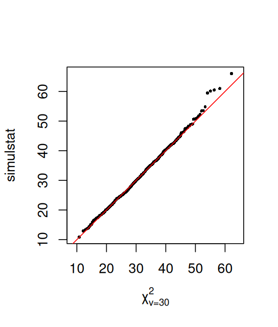

Figure 2.8: Our simulated statistic’s distribution compared to \(\chi_{30}^2\) using a quantile-quantile (QQ) plot, which shows the theoretical quantiles for the \(\chi^2_{30}\) distribution on the horizontal axis and the sampled ones on the vertical axis.

Having convinced ourselves that simulstat is well described by a \(\chi^2_{30}\) distribution, we can use that to compute our p-value, i.e., the probability that under the null hypothesis (counts are distributed as multinomial with probabilities \(p_{\text{A}} = 0.35\), \(p_{\text{C}} = 0.15\), \(p_{\text{G}} = 0.2\), \(p_{\text{T}} = 0.3\)) we observe a value as high as S1=70.1:

1 - pchisq(S1, df = 30)

[1] 4.74342e-05

With such a small p-value, the null hypothesis seems improbable. Note how this computation did not require the 1000 simulations and was faster.

2.7 Chargaff’s Rule

The most important pattern in the nucleotide frequencies was discovered by Chargaff (Elson and Chargaff 1952).

Long before DNA sequencing was available, using the weight of the molecules, he asked whether the nucleotides occurred at equal frequencies. He called this the tetranucleotide hypothesis. We would translate that into asking whether \(p_{\text{A}} = p_{\text{C}} = p_{\text{G}} = p_{\text{T}}\).

Unfortunately, Chargaff only published the percentages of the mass present in different organisms for each of the nucleotides, not the measurements themselves.

load("../data/ChargaffTable.RData")
ChargaffTable

                  A    T    C    G
Human-Thymus   30.9 29.4 19.9 19.8
Mycobac.Tuber  15.1 14.6 34.9 35.4
Chicken-Eryth. 28.8 29.2 20.5 21.5
Sheep-liver    29.3 29.3 20.5 20.7
Sea Urchin     32.8 32.1 17.7 17.3
Wheat          27.3 27.1 22.7 22.8
Yeast          31.3 32.9 18.7 17.1
E.coli         24.7 23.6 26.0 25.7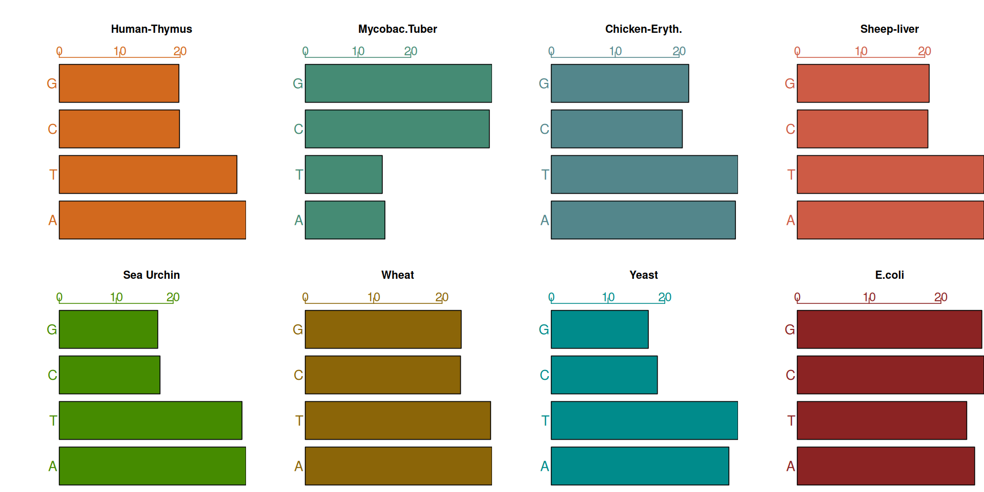

Figure 2.9: Barplots for the different rows in ChargaffTable. Can you spot the pattern?

Question 2.13

• Do these data seem to come from equally likely multinomial categories?

• Can you suggest an alternative pattern? puted from simulations u

• Can you do a quantitative analysis of the pattern, perhaps inspired by the simulations above?

Solution

Chargaff saw the answer to this question and postulated a pattern called base pairing, which ensured a perfect match of the amount of adenine (A) in the DNA of an organism to the amount of thymine (T). Similarly, whatever the amount of guanine (G), the amount of cytosine (C) would be the same. This is now called Chargaff’s rule. On the other hand, the amount of C/G in an organism could be quite different from that of A/T, with no obvious pattern across organisms. Based on Chargaff’s rule, we might define a statistic

\[ (p_{\text{C}} - p_{\text{G}})^2 + (p_{\text{A}} - p_{\text{T}})^2, \]

summed over all rows of the table. We are going to look at a comparison between the data and what would occur if the nucleotides were ‘exchangeable’, in the sense that the probabilities observed in each row were in no particular order, so that there were no special relationship between the proportions of As and Ts, or between those of Cs and Gs.

statChf = function(x){
  sum((x[, "C"] - x[, "G"])^2 + (x[, "A"] - x[, "T"])^2)
}
chfstat = statChf(ChargaffTable)
permstat = replicate(100000, {
     permuted = t(apply(ChargaffTable, 1, sample))
     colnames(permuted) = colnames(ChargaffTable)
     statChf(permuted)
})
pChf = mean(permstat <= chfstat)
pChf

[1] 0.00014

hist(permstat, breaks = 100, main = "", col = "lavender")
abline(v = chfstat, lwd = 2, col = "red")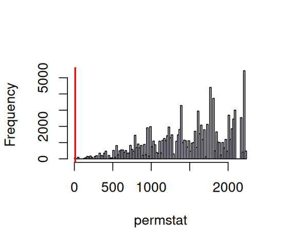

Figure 2.10: Histogram of our statistic statChf computed from simulations using per-row permutations of the columns. The value it yields for the observed data is shown by the red line.

The histogram in Figure 2.10 shows that it is quite rare to have a value as small as the observed 11.1, where the red line is drawn. The probability of observing a value as small or smaller is pChf=1.4^{-4}. Thus the data strongly support Chargaff’s insight.

Question 2.14

When computing pChf, we only looked at the values in the null distribution smaller than the observed value. Why did we do this in a one-sided way here?

2.7.1 Two categorical variables

Up to now, we have visited cases where the data are taken from a sample that can be classified into different boxes: the binomial for Yes/No binary boxes and the multinomial distribution for categorical variables such as A, C, G, T or different genotypes such aa, aA, AA. However it might be that we measure two (or more) categorical variables on a set of subjects, for instance eye color and hair color. We can then cross-tabulate the counts for every combination of eye and hair color. We obtain a table of counts called a contingency table. This concept is very useful for many biological data types.

HairEyeColor[,, "Female"]

       Eye
Hair    Brown Blue Hazel Green
  Black    36    9     5     2
  Brown    66   34    29    14
  Red      16    7     7     7
  Blond     4   64     5     8

Question 2.15

Explore the HairEyeColor object in R. What data type, shape and dimensions does it have?

Solution

It is a numeric array with three dimensions:

str(HairEyeColor)

 'table' num [1:4, 1:4, 1:2] 32 53 10 3 11 50 10 30 10 25 ...
 - attr(*, "dimnames")=List of 3
  ..$ Hair: chr [1:4] "Black" "Brown" "Red" "Blond"
  ..$ Eye : chr [1:4] "Brown" "Blue" "Hazel" "Green"
  ..$ Sex : chr [1:2] "Male" "Female"

## ?HairEyeColor

Color blindness and sex

Deuteranopia is a form of red-green color blindness due to the fact that medium wavelength sensitive cones (green) are missing. A deuteranope can only distinguish 2 to 3 different hues, whereas somebody with normal vision sees 7 different hues. A survey for this type of color blindness in human subjects produced a two-way table crossing color blindness and sex.

load("../data/Deuteranopia.RData")
Deuteranopia

          Men Women
Deute      19     2
NonDeute 1981  1998

How do we test whether there is a relationship between sex and the occurrence of color blindness? We postulate the null model with two independent binomials: one for sex and one for color blindness. Under this model we can estimate all the cells’ multinomial probabilities, and we can compare the observed counts to the expected ones. This is done through the chisq.test function in R.

chisq.test(Deuteranopia)

    Pearson's Chi-squared test with Yates' continuity correction

data:  Deuteranopia
X-squared = 12.255, df = 1, p-value = 0.0004641

The small p value tells us that we should expect to see such a table with only a very small probability under the null model – i.e., if the fractions of deuteranopic color blind among women and men were the same.

We’ll see another test for this type of data called Fisher’s exact test (also known as the hypergeometric test) in Section 10.3.2. This test is widely used for testing the over-representations of certain types of genes in a list of significantly expressed ones.

2.7.2 A special multinomial: Hardy-Weinberg equilibrium

Here we highlight the use of a multinomial with three possible levels created by combining two alleles M and N. Suppose that the overall frequency of allele M in the population is \(p\), so that of N is \(q = 1-p\). The Hardy-Weinberg model looks at the relationship between \(p\) and \(q\) if there is independence of the frequency of both alleles in a genotype, the so-called Hardy-Weinberg equilibrium (HWE). This would be the case if there is random mating in a large population with equal distribution of the alleles among sexes. The probabilities of the three genotypes are then as follows:

\[ p_{\text{MM}}=p^2,\quad p_{\text{NN}}=q^2,\quad p_{\text{MN}}=2pq \tag{2.5}\]

We only observe the frequencies \((n_{\text{MM}},\,n_{\text{MN}},\,n_{\text{NN}})\) for the genotypes MM, MN, NN and the total number \(S=n_{\text{MM}}+ n_{\text{MN}}+n_{\text{NN}}\). We can write the likelihood, i.e., the probability of the observed data when the probabilities of the categories are given by Equation 2.5, using the multinomial formula

\[ P(n_{\text{MM}},\,n_{\text{MN}},\,n_{\text{NN}}\;|\;p) = {S \choose n_{\text{MM}},n_{\text{MN}},n_{\text{NN}}} (p^2)^{n_{\text{MM}}} \,\times\, (2pq)^{n_{\text{MN}}} \,\times\, (q^2)^{n_{\text{NN}}}, \]

and the log-likelihood under HWE

\[ L(p)=n_{\text{MM}}\log(p^2)+n_{\text{MN}} \log(2pq)+n_{\text{NN}}\log(q^2). \]

The value of \(p\) that maximizes the log-likelihood is

\[ p = \frac{n_{\text{MM}} + n_{\text{MN}}/2}{S}. \]

See (Rice 2006, chap. 8, Section 5) for the proof. Given the data \((n_{\text{MM}},\,n_{\text{MN}},\,n_{\text{NN}})\), the log-likelihood \(L\) is a function of only one parameter, \(p\). Figure 2.11 shows this log-likelihood function for different values of \(p\) for the 216th row of the Mourant data⁷, computed in the following code.

⁷ This is genotype frequency data of blood group alleles from Mourant, Kopec, and Domaniewska-Sobczak (1976) available through the R package HardyWeinberg.

library("HardyWeinberg")
data("Mourant")
Mourant[214:216,]

    Population    Country Total  MM  MN  NN
214    Oceania Micronesia   962 228 436 298
215    Oceania Micronesia   678  36 229 413
216    Oceania     Tahiti   580 188 296  96

nMM = Mourant$MM[216]
nMN = Mourant$MN[216]
nNN = Mourant$NN[216]
loglik = function(p, q = 1 - p) {
  2 * nMM * log(p) + nMN * log(2*p*q) + 2 * nNN * log(q)
}
xv = seq(0.01, 0.99, by = 0.01)
yv = loglik(xv)
plot(x = xv, y = yv, type = "l", lwd = 2,
     xlab = "p", ylab = "log-likelihood")
imax = which.max(yv)
abline(v = xv[imax], h = yv[imax], lwd = 1.5, col = "blue")
abline(h = yv[imax], lwd = 1.5, col = "purple")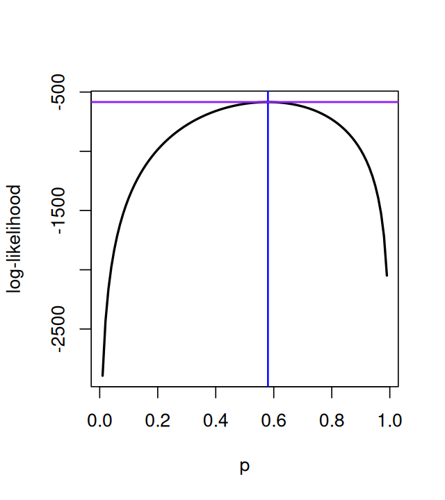

Figure 2.11: Plot of the log-likelihood for the Tahiti data.

The maximum likelihood estimate for the probabilities in the multinomial is also obtained by using the observed frequencies as in the binomial case, however the estimates have to account for the relationships between the three probabilities. We can compute \(\hat{p}_{\text{MM}}\), \(\hat{p}_{\text{MN}}\) and \(\hat{p}_{\text{NN}}\) using the af function from the HardyWeinberg package.

phat  =  af(c(nMM, nMN, nNN))
phat

        A 
0.5793103 

pMM   =  phat^2
qhat  =  1 - phat

The expected values under Hardy-Weinberg equilibrium are then

pHW = c(MM = phat^2, MN = 2*phat*qhat, NN = qhat^2)
sum(c(nMM, nMN, nNN)) * pHW

    MM.A     MN.A     NN.A 
194.6483 282.7034 102.6483 

which we can compare to the observed values above. We can see that they are quite close to the observed values. We could further test whether the observed values allow us to reject the Hardy-Weinberg model, either by doing a simulation or a \(\chi^2\) test as above. A visual evaluation of the goodness-of-fit of Hardy-Weinberg was designed by de Finetti (Finetti 1926; Cannings and Edwards 1968). It places every sample at a point whose coordinates are given by the proportions of each of the different alleles.

Visual comparison to the Hardy-Weinberg equilibrium

We use the HWTernaryPlot function to display the data and compare it to Hardy-Weinberg equilibrium graphically.

pops = c(1, 69, 128, 148, 192)
genotypeFrequencies = as.matrix(Mourant[, c("MM", "MN", "NN")])
HWTernaryPlot(genotypeFrequencies[pops, ],
        markerlab = Mourant$Country[pops],
        alpha = 0.0001, curvecols = c("red", rep("purple", 4)),
        mcex = 0.75, vertex.cex = 1)

Figure 2.12: This de Finetti plot shows the points as barycenters of the three genotypes using the frequencies as weights on each of the corners of the triangle. The Hardy-Weinberg model is the red curve, the acceptance region is between the two purple lines. We see that the US is the furthest from being in HW equilibrium.

Question 2.16

Make the ternary plot as in the code above, then add the other data points to it, what do you notice? You could back up your discussion using the HWChisq function.

Solution

HWTernaryPlot(genotypeFrequencies[-pops, ], 
              newframe = FALSE, alpha = 0.0001, cex = 0.5)

Question 2.17

Divide all total frequencies by 50, keeping the same proportions for each of the genotypes, and recreate the ternary plot.

• What happens to the points ?

• What happens to the confidence regions and why?

Solution

newgf = round(genotypeFrequencies / 50)
HWTernaryPlot(newgf[pops, ],
              markerlab = Mourant$Country[pops],
              curvecols = c("red", rep("purple", 4)),
              alpha = 0.0001, mcex = 0.75, vertex.cex = 1)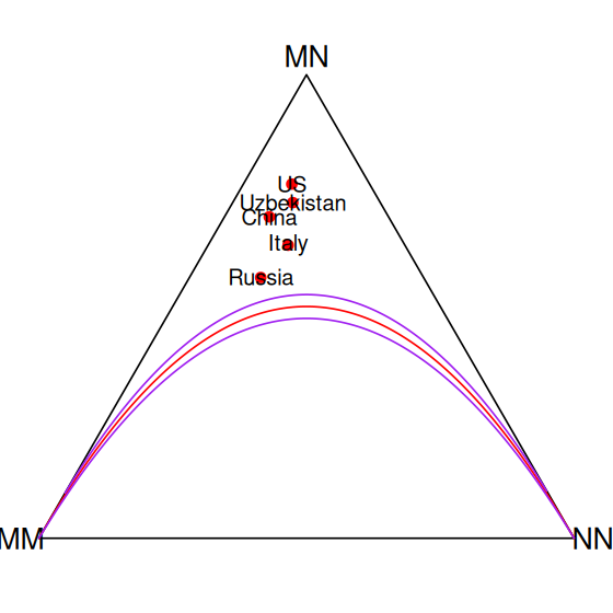

2.7.3 Concatenating several multinomials: sequence motifs and logos

The Kozak Motif is a sequence that occurs close to the start codon ATG of a coding region. The start codon itself always has a fixed spelling but in positions 5 to the left of it, there is a nucleotide pattern in which the letters are quite far from being equally likely.

We summarize this by giving the position weight matrix (PWM) or position-specific scoring matrix (PSSM), which provides the multinomial probabilities at every position. This is encoded graphically by the sequence logo (Figure 2.13).

library("seqLogo")
load("../data/kozak.RData")
kozak

  [,1] [,2] [,3] [,4] [,5] [,6] [,7] [,8] [,9]
A 0.33 0.25  0.4 0.15 0.20    1    0    0 0.05
C 0.12 0.25  0.1 0.40 0.40    0    0    0 0.05
G 0.33 0.25  0.4 0.20 0.25    0    0    1 0.90
T 0.22 0.25  0.1 0.25 0.15    0    1    0 0.00

pwm = makePWM(kozak)
seqLogo(pwm, ic.scale = FALSE)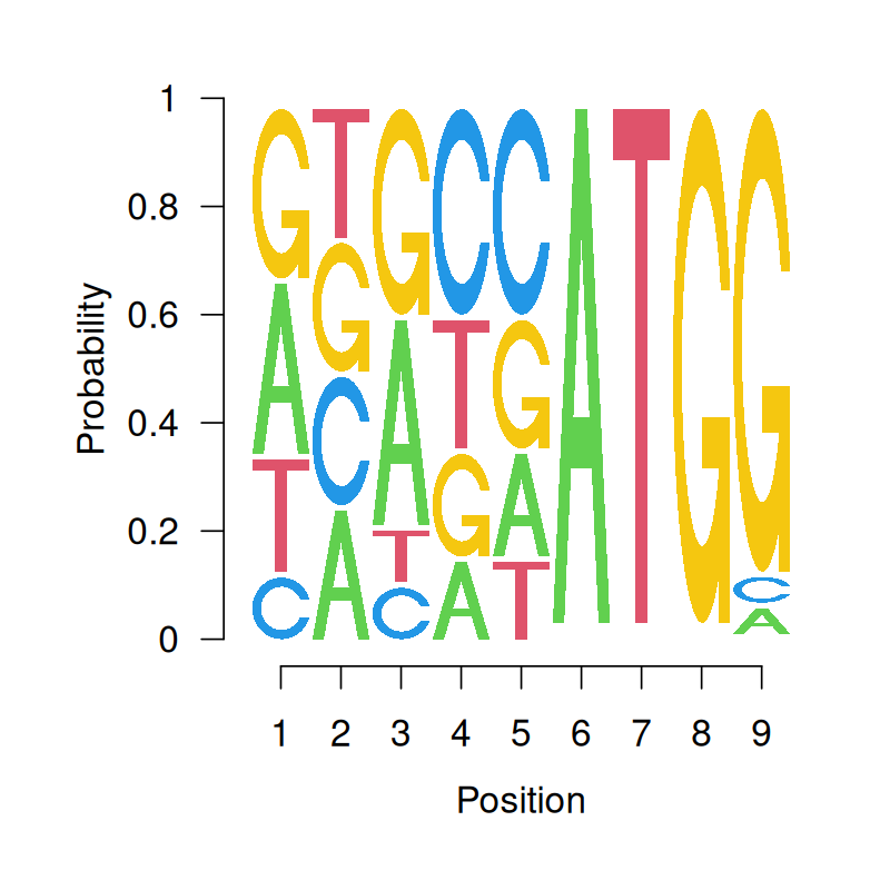

Figure 2.13: Here is a diagram called a sequence logo for the position dependent multinomial used to model the Kozak motif. It codifies the amount of variation in each of the positions on a log scale. The large letters represent positions where there is no uncertainty about which nucleotide occurs.

Over the last sections, we’ve seen how the different “boxes” in the multinomial distributions we have encountered very rarely have equal probabilities. In other words, the parameters \(p_1, p_2, ...\) are often different, depending on what is being modeled. Examples of multinomials with unequal frequencies include the twenty different amino acids, blood types and hair color.

If there are multiple categorical variables, we have seen that they are rarely independent (sex and colorblindness, hair and eye color, …). We will see later in Chapter 9 that we can explore the patterns in these dependencies by using multivariate decompositions of the contingency tables. Here, we’ll look at an important special case of dependencies between categorical variables: those that occur along a sequence (or “chain”) of categorical variables, e.g., over time or along a biopolymer.

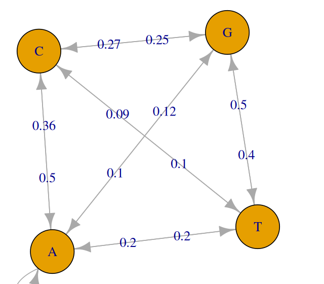
2.8 Modeling sequential dependencies: Markov chains

If we want to predict tomorrow’s weather, a reasonably good guess is that it will most likely be the same as today’s weather, in addition we may state the probabilities for various kinds of possible changes^[The same reasoning can also be applied in reverse: we could “predict” yesterday’s weather from today’s.. This method for weather forecasting is an example for the Markov assumption: the prediction for tomorrow only depends on the state of things today, but not on yesterday or three weeks ago (all information we could potentially use is already contained in today’s weather). The weather example also highlights that such an assumption need not necessarily be exactly true, but it should be a good enough assumption. It is fairly straightforward to extend this assumption to dependencies on the previous \(k\) days, where \(k\) is a finite and hopefully not too large number. The essence of the Markov assumption is that the process has a finite “memory”, so that predictions only need to look back for a finite amount of time.

Instead of temporal sequences, we can also apply this to biological sequences. In DNA, we may see specific succession of patterns so that pairs of nucleotides, called digrams, say, [CG, CA, CC] and [CT] are not equally frequent. For instance, in parts of the genome we see more frequent instances of [CA] than we would expect under independence:

\[ P(\mathtt{CA}) \neq P(\mathtt{C}) \, P(\mathtt{A}). \]

We model this dependency in the sequence as a Markov chain:

\[ P(\mathtt{CA}) = P(\mathtt{NCA}) = P(\mathtt{NNCA}) = P(...\mathtt{CA}) = P(\mathtt{C}) \, P(\mathtt{A|C}), \]

where N stands for any nucleotide, and \(P(\mathtt{A|C})\) stands for “the probability of \(\mathtt{A}\), given that the preceding base is a \(\mathtt{C}\)”. Figure 2.14 shows a schematic representation of such transitions on a graph.

Figure 2.14: Visualisation of a 4-state Markov chain. The probability of each possible digram (e.,g., CA) is given by the weight of the edge between the corresponding nodes. So for instance, the probability of CA is given by the edge C$ o$ A. We’ll see in Chapter 11 how to use R packages to draw these type of network graphs.

2.9 Bayesian Thinking

Figure 2.15: Turtles all the way down. Bayesian modeling of the uncertainty of the parameter of a distribution is done by using a random variable whose distribution may depend on parameters whose uncertainty can be modeled as a random variable; these are called hierarchical models.

Up to now we have followed a classical approach, where the parameters of our models and the distributions they use, i.e., the probabilities of the possible different outcomes, represent long term frequencies. The parameters are—at least conceptually—definite, knowable and fixed. We may not know them, so we estimate them from the data at hand. However, such an approach does not take into account any information that we might already have, and that might inform us on the parameters or make certain parameter values or their combinations more likely than others—even before we see any of the current set of data. For that we need a different approach, in which we use probabilistic models (i.e., distributions) to express our prior knowledge⁸ about the parameters, and use the current data to update such knowledge, for instance by shifting those distributions or making them more narrow. Such an approach is provided by the Bayesian paradigm (Figure 2.15).

⁸ Some like to say “our belief(s)”.

The Bayesian paradigm is a practical approach where prior and posterior distributions to model our knowledge before and after collecting some data and making an observation. It can be iterated ad infinitum: the posterior after one round of data generation can be used as the prior for the next round. Thus, it is also particularly useful for integrating or combining information from different sources.

The same idea can also be applied to hypothesis testing, where we want to use data to decide whether we believe that a certain statement—which we might call the hypothesis \(H\)—is true. Here, our “parameter” is the probability that \(H\) is true, and we can formalize our prior knowledge in the form of a prior probability, written \(P(H)\)⁹. After we see the data, we have the posterior probability. We write it as \(P(H\,|\,D)\), the probability of \(H\) given that we saw \(D\). This may be higher or lower than \(P(H)\), depending on what the data \(D\) were.

⁹ For a so-called frequentist, such a probability does not exist. Their viewpoint is that, although the truth is unknown, in reality the hypothesis is either true or false; there is no meaning in calling it, say, “70% true”.

2.9.1 Example: haplotype frequencies

To keep the mathematical formalism to a minimum, we start with an example from forensics, using combined signatures (haplotypes) from the Y chromosome.

A haplotype is a collection of alleles (DNA sequence variants) that are spatially adjacent on a chromosome, are usually inherited together (recombination tends not to disconnect them), and thus are genetically linked. In this case we are looking at linked variants on the Y chromosome.

First we’ll look at the motivation behind haplotype frequency analyses, then we’ll revisit the idea of likelihood. After this, we’ll explain how we can think of unknown parameters as being random numbers themselves, modeling their uncertainty with a prior distribution. Then we will see how to incorporate new data observed into the probability distributions and compute posterior confidence statements about the parameters.

Figure 2.16: A short tandem repeat (STR) in DNA occurs when a pattern of two or more nucleotides is repeated, and the repeated sequences are directly adjacent to each other. An STR is also known as a microsatellite. The pattern can range in length from 2 to 13 nucleotides, and the number of repeats is highly variable across individuals. STR numbers can be used as genetic signatures.

Figure 2.17: Location of short tandem repeats (STR) on the human Y chromosome. Source: https://strbase.nist.gov/ystrpos1.htm

Figure 2.18: Y STR haplotype lookup from a database used by the FBI.

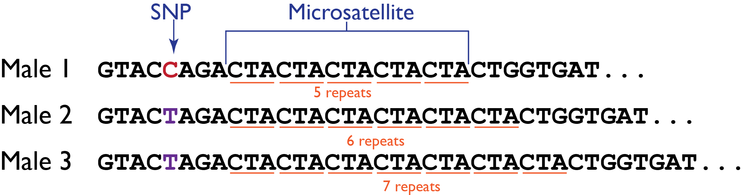
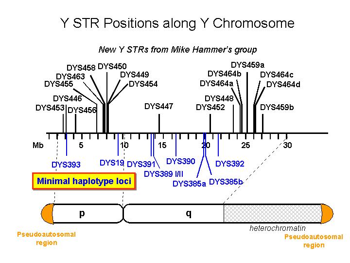
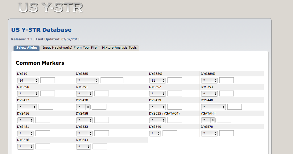
We’re interested in the frequencies of particular Y-haplotypes that consist of a set of different short tandem repeats (STR). The combination of STR numbers at the specific locations used for DNA forensics are labeled by the number of repeats at the specific positions. Here is a short excerpt of such an STR haplotype table:

haplo6 = read.table("../data/haplotype6.txt", header = TRUE)
haplo6

  Individual DYS19 DXYS156Y DYS389m DYS389n DYS389p
1         H1    14       12       4      12       3
2         H3    15       13       4      13       3
3         H4    15       11       5      11       3
4         H5    17       13       4      11       3
5         H7    13       12       5      12       3
6         H8    16       11       5      12       3

The table says that the haplotype H1 has 14 repeats at position DYS19, 12 repeats at position DXYS156Y, etc. Suppose we want to find the underlying proportion \(p\) of a particular haplotype in a population of interest, by haplotyping \(n=300\) men; and suppose we found H1 in \(y=40\) of them. We are going to use the binomial distribution \(B(n,p)\) to model this, with \(p\) unknown.

The haplotypes created through the use of these Y-STR profiles are shared between men in the same patriarchal lineages. Thus, it is possible that two different men share the same profile.

2.9.2 Simulation study of the Bayesian paradigm for the binomial distribution

Instead of assuming that our parameter \(p\) has one single value (e.g., the maximum likelihood estimate 40/300), the Bayesian approach allows us to see it as a draw from a statistical distribution. The distribution expresses our belief about the possible values of the parameter \(p\). In principle, we can use any distribution that we like whose possible values are permissible for \(p\). As here we are looking at a parameter that expresses a proportion or a probability, and which takes its values between 0 and 1, it is convenient to use the Beta distribution. Its density formula is written

\[ f_{\alpha,\beta}(x) = \frac{x^{\alpha-1}\,(1-x)^{\beta-1}}{\text{B}(\alpha,\beta)}\quad\text{where}\quad \text{B}(\alpha,\beta)=\frac{\Gamma(\alpha)\Gamma(\beta)}{\Gamma(\alpha+\beta)}. \tag{2.6}\]

We can see in Figure 2.19 how this function depends on two parameters \(\alpha\) and \(\beta\), which makes it a very flexible family of distributions (it can “fit” a lot different situations). And it has a nice mathematical property: if we start with a prior belief on \(p\) that is Beta-shaped, observe a dataset of \(n\) binomial trials, then update our belief, the posterior distribution on \(p\) will also have a Beta distribution, albeit with updated parameters. This is a mathematical fact. We will not prove it here, however we demonstrate it by simulation.

Figure 2.19: Beta distributions with \(\alpha=10,20,50\) and \(\beta=30,60,150\). We can use these as a prior for probability of success in a binomial experiment. These three distributions have the same mean (\(\frac{\alpha}{\alpha +\beta}\)), but different concentrations around the mean.

2.9.3 The distribution of \(Y\)

For a given choice of \(p\), we know what the distribution of \(Y\) is, by virtue of Equation 2.3. But what is the distribution of \(Y\) if \(p\) itself also varies according to some distribution? We call this the marginal distribution of \(Y\). Let’s simulate that. First we generate a random sample rp of 100000 \(p\)s. For each of them, we then generate a random sample of \(Y\), shown in Figure 2.20. In the code below, for the sake of demonstration we use the parameters 50 and 350 for the prior. Such a prior is already quite informative (“peaked”) and may, e.g., reflect beliefs we have based on previous studies. In Question 2.20 you have the opportunity to try out a “softer” (less informative) prior. We again use vapply to apply a function, the unnamed (anonymous) function of x, across all elements of rp to obtain as a result another vector y of the same length.

rp = rbeta(100000, 50, 350)
y = vapply(rp, 
           function(x) rbinom(1, prob = x, size = 300), 
           integer(1))
hist(y, breaks = 50, col = "orange", main = "", xlab = "")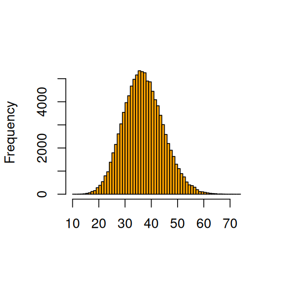

Figure 2.20: Marginal Distribution of \(Y\).

Question 2.18

Verify that we could have gotten the same result as in the above code chunk by using R’s vectorisation capabilities and writing rbinom(length(rp), rp, size = 300).

Solution

set.seed(0xbebe)
y1 = vapply(rp, 
            function(x) rbinom(1, prob = x, size = 300), 
            integer(1))
set.seed(0xbebe)
y2 = rbinom(length(rp), rp, size = 300)
stopifnot(identical(y1, y2))

2.9.4 Histogram of all the \(p\)s such that \(Y=40\): the posterior distribution

So now let’s compute the posterior distribution of \(p\) by conditioning on those outcomes where \(Y\) was 40. We compare it to the theoretical posterior, densPostTheory, of which more below. The results are shown in Figure 2.21.

pPostEmp = rp[ y == 40 ]
hist(pPostEmp, breaks = 40, col = "chartreuse4", main = "",
  probability = TRUE, xlab = "posterior p")

p_seq = seq(0, 1, by = 0.001)
densPostTheory = dbeta(p_seq, 50 + 40, 350 + 260)
lines(p_seq, densPostTheory, type = "l", lwd = 3)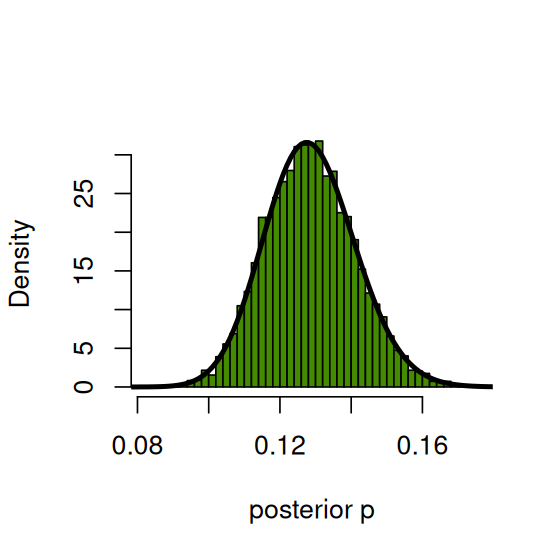

Figure 2.21: Only choosing the values of the distribution with \(Y=40\) gives the posterior distribution of \(p\). The histogram (green) shows the simulated values for the posterior distribution, the line the density of a Beta distribution with the theoretical parameters.

We can also check the means of both distributions computed above and see that they are close to 4 significant digits.

mean(pPostEmp)

[1] 0.1285996

dp = p_seq[2] - p_seq[1]
sum(p_seq * densPostTheory * dp)

[1] 0.1285714

To approximate the mean of the theoretical density densPostTheory, we have above literally computed the integral

\[ \int_0^1 p \, f(p) \, dp \]

using numerical integration, i.e., the sum over the integral. This is not always convenient (or feasible), in particular if our model involves not just a single, scalar parameter \(p\), but has many parameters, so that we are dealing with a high-dimensional parameter vector and a high-dimensional integral. If the integral cannot be computed analytically, we can use Monte Carlo integration. You already saw a very simple instance of Monte Carlo integration in the code above, where we sampled the posterior with pPostEmp and performed integration to compute the posterior mean by calling R’s mean function. In this case, an alternative Monte Carlo algorithm is to generate posterior samples using the rbeta function directly with the right parameters.

pPostMC = rbeta(n = 100000, 90, 610)
mean(pPostMC)

[1] 0.1285695

We can check the concordance between the Monte Carlo samples pPostMC and pPostEmp, generated in slightly different ways, using a quantile-quantile plot (QQ-plot, Figure 2.22).

qqplot(pPostMC, pPostEmp, type = "l", asp = 1)
abline(a = 0, b = 1, col = "blue")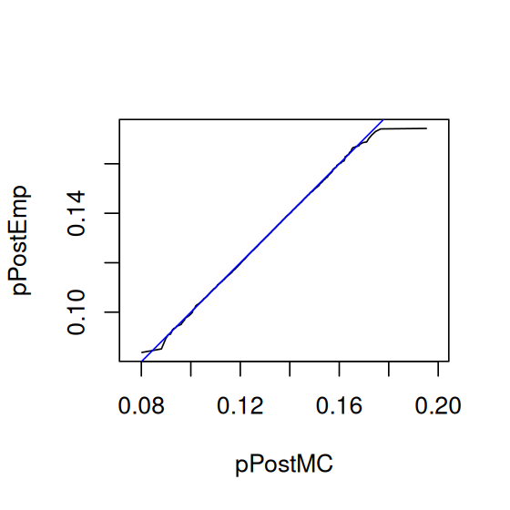

Figure 2.22: Quantile-quantile (QQ) plot of our Monte Carlo sample pPostMC from the theoretical distribution and our simulation sample pPostEmp. We could also similarly compare either of these two distributions to the theoretical distribution function pbeta(., 90, 610). If the curve lies on the line \(y=x\), this indicates a good agreement. There are some random differences at the tails.

Question 2.19

What is the difference between the simulation that results in pPostEmp and the Monte Carlo simulation that leads to pPostMC?

2.9.5 The posterior distribution is also a Beta

Now we have seen that the posterior distribution is also a Beta. In our case its parameters \(\alpha=90\) and \(\beta=610\) were obtained by summing the prior parameters \(\alpha=50\), \(\beta=350\) with the observed successes \(y=40\) and the observed failures \(n-y=260\), thus obtaining the posterior

\[ \text{Beta}(90,\, 610)=\text{Beta}(\alpha+y,\text{Beta}+(n-y)). \]

We can use it to give the best¹⁰ estimate we can for \(p\) with its uncertainty given by the posterior distribution.

¹⁰ We could take the value that maximizes the posterior distribution as our best estimate, this is called the MAP estimate, and in this case it would be \(\frac{\alpha-1}{\alpha+\beta-2}=\frac{89}{698}\doteq 0.1275\).

2.9.6 Suppose we had a second series of data

After seeing our previous data, we now have a new prior, \(\text{Beta}(90, 610)\). Suppose we collect a new set of data with \(n=150\) observations and \(y=25\) successes, thus 125 failures. Now what would we take to be our best guess at \(p\)?

Using the same reasoning as before, the new posterior will be \(\text{Beta}(90+25=115,\, 610+125=735)\). The mean of this distribution is \(\frac{115}{115+735}=\frac{115}{850}\simeq 0.135\), thus one estimate of \(p\) would be 0.135. The maximum a posteriori (MAP) estimate would be the mode of \(\text{Beta}(115, 735)\), ie \(\frac{114}{848}\simeq 0.134\). Let’s check this numerically.

densPost2 = dbeta(p_seq, 115, 735)
mcPost2   = rbeta(1e6, 115, 735)
sum(p_seq * densPost2 * dp)   # mean, by numeric integration

[1] 0.1352941

mean(mcPost2)                 # mean by MC

[1] 0.1352655

p_seq[which.max(densPost2)]   # MAP estimate

[1] 0.134

Question 2.20

Redo all the computations replacing our original prior with a softer prior (less peaked), meaning that we use less prior information. For instance, try Beta(1,1), which is the uniform distribution. How much does this change the final result?

As a general rule, the prior rarely changes the posterior distribution substantially except if it is very peaked. This would be the case if, at the outset, we were already rather sure of what to expect. Another case when the prior has an influence is if there is very little data.

The best situation to be in is to have enough data to swamp the prior so that its choice doesn’t have much impact on the final result.

2.9.7 Confidence Statements for the proportion parameter

Now it is time to conclude about what the proportion \(p\) actually is, given the data. One summary is a posterior credibility interval, which is a Bayesian analog of the confidence interval. We can take the 2.5 and 97.5-th percentiles of the posterior distribution: \(P(q_{2.5\%} \leq p \leq q_{97.5\%})=0.95\).

quantile(mcPost2, c(0.025, 0.975))

     2.5%     97.5% 
0.1131068 0.1590214 

Figure 2.23: An example from Love, Huber, and Anders (2014) shows plots of the likelihoods (solid lines, scaled to integrate to 1) and the posteriors (dashed lines) for the green and purple genes and of the prior (solid black line): due to the higher dispersion of the purple gene, its likelihood is wider and less peaked (indicating less information), and the prior has more influence on its posterior than for the green gene. The stronger curvature of the green posterior at its maximum translates to a smaller reported standard error for the MAP logarithmic fold change (LFC) estimate (horizontal error bar).

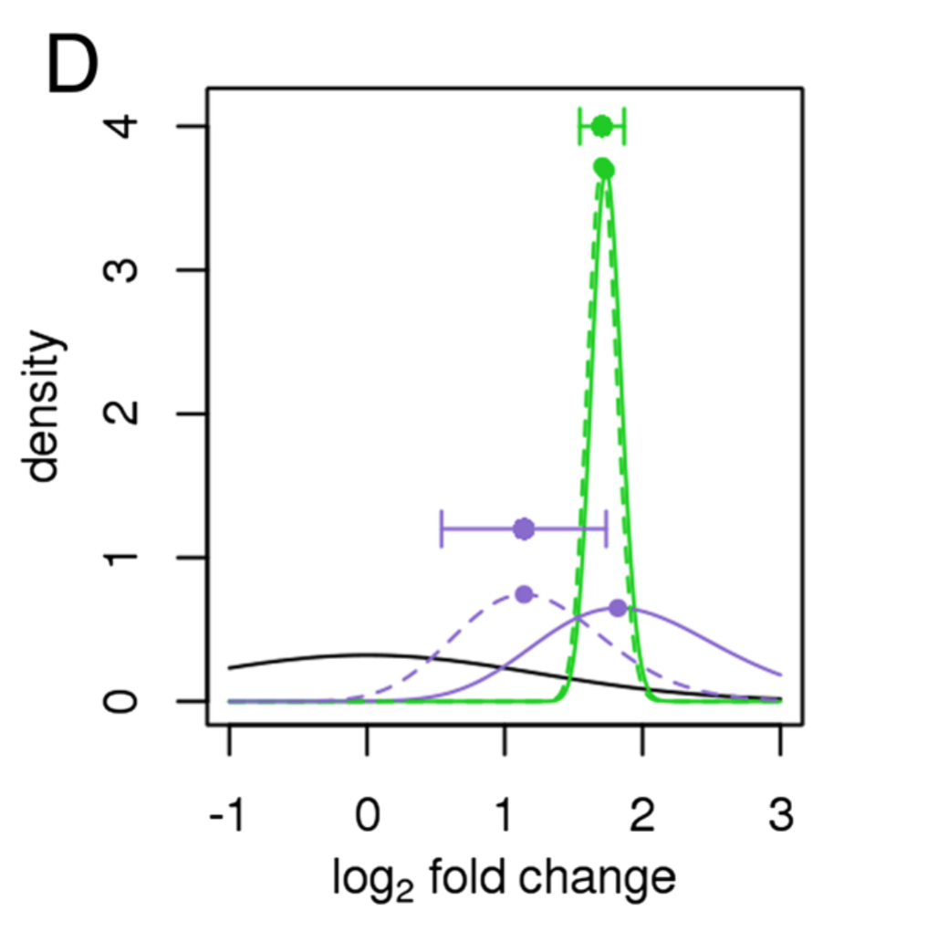
2.10 Example: occurrence of a nucleotide pattern in a genome

The examples we have seen up to now have concentrated on distributions of discrete counts and categorical data. Let’s look at an example of distributions of distances, which are quasi-continuous. This case study of the distributions of the distances between instances of a specific motif in genome sequences will also allow us to explore specific genomic sequence manipulations in Bioconductor.

The Biostrings package provides tools for working with sequence data. The essential data structures, or classes as they are known in R, are DNAString and DNAStringSet. These enable us to work with one or multiple DNA sequences efficiently .

The Biostrings package also contains additional classes for representing amino acid sequences, and more general, biology-inspired sequences.

library("Biostrings")

Question 2.21

Explore some of the useful data and functions provided in the Biostrings package by exploring the tutorial vignette.

Solution

The first line prints genetic code information, the second one returns IUPAC nucleotide ambiguity codes. The third line lists all the vignettes available in the Biostrings package, the fourth display one particular vignette.

GENETIC_CODE
IUPAC_CODE_MAP
vignette(package = "Biostrings")
vignette("BiostringsQuickOverview", package = "Biostrings")

This last command will open a list in your browser window from which you can access the documentation¹¹. The BSgenome package provides access to many genomes, and you can access the names of the data packages that contain the whole genome sequences by typing

¹¹ Vignettes are manuals for the packages complete with examples and case studies.

library("BSgenome")
ag = available.genomes()
length(ag)

[1] 113

ag[1:2]

[1] "BSgenome.Alyrata.JGI.v1"              
[2] "BSgenome.Amellifera.BeeBase.assembly4"

We are going to explore the occurrence of the AGGAGGT motif¹² in the genome of E.coli. We use the genome sequence of one particular strain, Escherichia coli str. K12 substr.DH10B¹³, whose NCBI accession number is NC_010473.

¹² This is the Shine-Dalgarno motif which helps initiate protein synthesis in bacteria.

¹³ It is known as the laboratory workhorse, often used in experiments.

library("BSgenome.Ecoli.NCBI.20080805")
Ecoli
shineDalgarno = "AGGAGGT"
ecoli = Ecoli$NC_010473

We can count the pattern’s occurrence in windows of width 50000 using the countPattern function.

window = 50000
starts = seq(1, length(ecoli) - window, by = window)
ends   = starts + window - 1
numMatches = vapply(seq_along(starts), function(i) {
  countPattern(shineDalgarno, ecoli[starts[i]:ends[i]],
               max.mismatch = 0)
  }, numeric(1))
table(numMatches)

numMatches
 0  1  2  3  4 
48 32  8  3  2 

Question 2.22

What distribution might this table fit ?

Solution

The Poisson is a good candidate, as a quantitative and graphical evaluation (see Figure 2.24) for these data shows.

library("vcd")
gf = goodfit(numMatches, "poisson")
summary(gf)

     Goodness-of-fit test for poisson distribution

                      X^2 df  P(> X^2)
Likelihood Ratio 4.134932  3 0.2472577

distplot(numMatches, type = "poisson")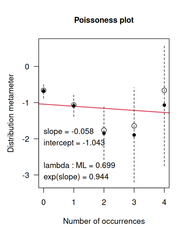

Figure 2.24: Evaluation of a Poisson model for motif counts along the sequence Ecoli$NC_010473.

We can inspect the matches using the matchPattern function.

sdMatches = matchPattern(shineDalgarno, ecoli, max.mismatch = 0)

You can type sdMatches in the R command line to obtain a summary of this object. It contains the locations of all 65 pattern matches, represented as a set of so-called views on the original sequence. Now what are the distances between them?

betweenmotifs = gaps(sdMatches)

So these are in fact the 66 complementary regions. Now let’s find a model for the distribution of the gap sizes between motifs. If the motifs occur at random locations, we expect the gap lengths to follow an exponential distribution¹⁴. The code below (whose output is shown in Figure 2.25) assesses this assumption. If the exponential distribution is a good fit, the points should lie roughly on a straight line. The exponential distribution has one parameter, the rate, and the line with slope corresponding to an estimate from the data is also shown.

¹⁴ How could we guess that the exponential is the right fit here? Whenever we have independent, random Bernoulli occurrences along a sequence, the gap lengths are exponential. You may be familiar with radioactive decay, where the waiting times between emissions are also exponentially distributed. It is a good idea if you are not familiar with this distribution to look up more details in the Wikipedia.

library("Renext")
expplot(width(betweenmotifs), rate = 1/mean(width(betweenmotifs)),
        labels = "fit")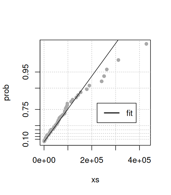

Figure 2.25: Evaluation of fit to the exponential distribution (black line) of the gaps between the motifs.

Question 2.23

There appears to be a slight deviation from the fitted line in Figure 2.25 at the right tail of the distribution, i.e., for the largest values. What could be the reason?

2.10.1 Modeling in the case of dependencies

As we saw in Section 2.8, nucleotide sequences are often dependent: the probability of seing a certain nucleotide at a given position tends to depend on the surrounding sequence. Here we are going to put into practice dependency modeling using a Markov chain. We are going to look at regions of chromosome 8 of the human genome and try to discover differences between regions called CpG¹⁵ islands and the rest.

¹⁵ CpG stands for 5’-C-phosphate-G-3’; this means that a C is connected to a G through a phosphate along the strand (this is unrelated to C-G base-pairing of Section 2.7). The cytosines in the CpG dinucleotide can be methylated, changing the levels of gene expression. This type of gene regulation is part of epigenetics. Some more information is on Wikipedia: CpG site and epigenetics.

We use data (generated by Irizarry, Wu, and Feinberg (2009)) that tell us where the start and end points of the islands are in the genome and look at the frequencies of nucleotides and of the digrams ‘CG’, ‘CT’, ‘CA’, ‘CC’. So we can ask whether there are dependencies between the nucleotide occurrences and if so, how to model them.

library("BSgenome.Hsapiens.UCSC.hg19")
chr8  =  Hsapiens$chr8
CpGtab = read.table("../data/model-based-cpg-islands-hg19.txt",
                    header = TRUE)
nrow(CpGtab)

[1] 65699

head(CpGtab)

    chr  start    end length CpGcount GCcontent pctGC obsExp
1 chr10  93098  93818    721       32       403 0.559  0.572
2 chr10  94002  94165    164       12        97 0.591  0.841
3 chr10  94527  95302    776       65       538 0.693  0.702
4 chr10 119652 120193    542       53       369 0.681  0.866
5 chr10 122133 122621    489       51       339 0.693  0.880
6 chr10 180265 180720    456       32       256 0.561  0.893

irCpG = with(dplyr::filter(CpGtab, chr == "chr8"),
         IRanges(start = start, end = end))

We use the :: operator to call the filter function specifically from the dplyr package—and not from any other packages that may happen to be loaded and defining functions of the same name. This precaution is particularly advisable in the case of the filter function, since this name is used by quite a few other packages. You can think of the normal (without ::) way of calling R functions like calling people by their first (given) names; whereas the fully qualified version with :: corresponds to calling someone by their full name. At least within the reach of the CRAN and Bioconductor repositories, such fully qualified names are guaranteed to be unique.

In the line above, we subset (filter) the data frame CpGtab to only chromosome 8, and then we create an IRanges object whose start and end positions are defined by the equally named columns of the data frame. In the IRanges function call (which constructs the object from its arguments), the first start is the argument name of the function, the second start refers to the column in the data frame obtained as an output from filter; and similarly for end. IRanges is a general container for mathematical intervals. We create the biological context¹⁶ with the next line.

¹⁶ The “I” in IRanges stands for “interval”; the “G” in GRanges for “genomic”.

grCpG = GRanges(ranges = irCpG, seqnames = "chr8", strand = "+")
genome(grCpG) = "hg19"

Now let’s visualize; see the output in Figure 2.26.

library("Gviz")
ideo = IdeogramTrack(genome = "hg19", chromosome = "chr8")
plotTracks(
  list(GenomeAxisTrack(),
    AnnotationTrack(grCpG, name = "CpG"), ideo),
    from = 2200000, to = 5800000,
    shape = "box", fill = "#006400", stacking = "dense")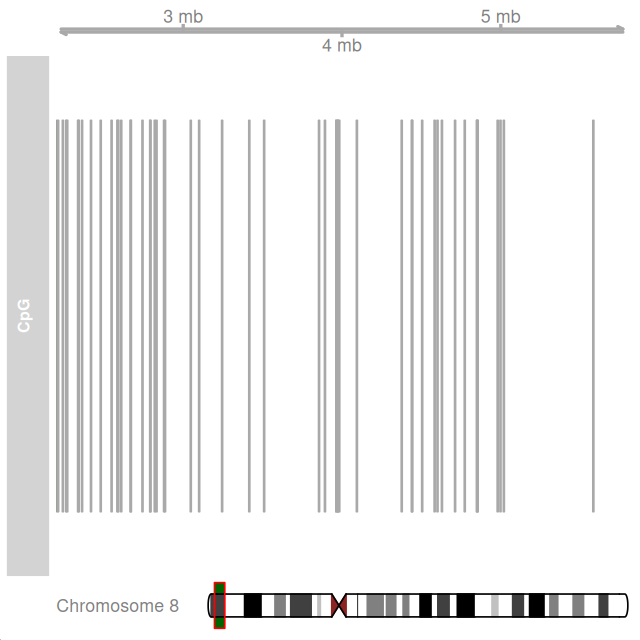

Figure 2.26: Gviz plot of CpG locations in a selected region of chromosome 8.

We now define so-called views on the chromosome sequence that correspond to the CpG islands, irCpG, and to the regions in between (gaps(irCpG)). The resulting objects CGIview and NonCGIview only contain the coordinates, not the sequences themselves (these stay in the big object Hsapiens$chr8), so they are fairly lightweight in terms of storage.

CGIview    = Views(unmasked(Hsapiens$chr8), irCpG)
NonCGIview = Views(unmasked(Hsapiens$chr8), gaps(irCpG))

We compute transition counts in CpG islands and non-islands using the data.

seqCGI      = as(CGIview, "DNAStringSet")
seqNonCGI   = as(NonCGIview, "DNAStringSet")
dinucCpG    = sapply(seqCGI, dinucleotideFrequency)
dinucNonCpG = sapply(seqNonCGI, dinucleotideFrequency)
dinucNonCpG[, 1]

 AA  AC  AG  AT  CA  CC  CG  CT  GA  GC  GG  GT  TA  TC  TG  TT 
389 351 400 436 498 560 112 603 359 336 403 336 330 527 519 485 

NonICounts = rowSums(dinucNonCpG)
IslCounts  = rowSums(dinucCpG)

For a four state Markov chain as we have, we define the transition matrix as a matrix where the rows are the from state and the columns are the to state.

TI  = matrix( IslCounts, ncol = 4, byrow = TRUE)
TnI = matrix(NonICounts, ncol = 4, byrow = TRUE)
dimnames(TI) = dimnames(TnI) =
  list(c("A", "C", "G", "T"), c("A", "C", "G", "T"))

We use the counts of numbers of transitions of each type to compute frequencies and put them into two matrices.

The transition probabilities are probabilities so the rows need to sum to 1.

MI = TI /rowSums(TI)
MI

           A         C         G         T
A 0.20457773 0.2652333 0.3897678 0.1404212
C 0.20128250 0.3442381 0.2371595 0.2173200
G 0.18657245 0.3145299 0.3450223 0.1538754
T 0.09802105 0.3352314 0.3598984 0.2068492

MN = TnI / rowSums(TnI)
MN

          A         C          G         T
A 0.3351380 0.1680007 0.23080886 0.2660524
C 0.3641054 0.2464366 0.04177094 0.3476871
G 0.2976696 0.2029017 0.24655406 0.2528746
T 0.2265813 0.1972407 0.24117528 0.3350027

Question 2.24

Are the transitions different in the different rows? This would mean that, for instance, \(P(\mathtt{A}\,|\,\mathtt{C}) \neq P(\mathtt{A}\,|\,\mathtt{T})\).

Solution

The transitions are different. For instance, the transitions from C to A and T to A for in the islands (MI) transition matrix seem very different (0.201 versus 0.098).

Question 2.25

Are the relative frequencies of the different nucleotides different in CpG islands compared to elsewhere?

Solution

freqIsl = alphabetFrequency(seqCGI, baseOnly = TRUE, collapse = TRUE)[1:4]
freqIsl / sum(freqIsl)

        A         C         G         T 
0.1781693 0.3201109 0.3206298 0.1810901 

freqNon = alphabetFrequency(seqNonCGI, baseOnly = TRUE, collapse = TRUE)[1:4]
freqNon / sum(freqNon)

        A         C         G         T 
0.3008292 0.1993832 0.1993737 0.3004139 

This shows an inverse pattern: in the CpG islands, C and G have frequencies around 0.32, whereas in the non-CpG islands, we have A and T that have frequencies around 0.30.

Question 2.26

How can we use these differences to decide whether a given sequence comes from a CpG island?

Solution

Use a \(\chi^2\) statistic to compare the frequencies between the observed and freqIsl and freqNon frequencies. For shorter sequences, this may not be sensitive enough, and a more sensitive approach is given below.

Given a sequence for which we do not know whether it is in a CpG island or not, we can ask what is the probability it belongs to a CpG island compared to somewhere else. We compute a score based on what is called the odds ratio. Let’s do an example: suppose our sequence \(x\) is ACGTTATACTACG, and we want to decide whether it comes from a CpG island or not.

If we model the sequence as a first order Markov chain we can write, supposing that the sequence comes from a CpG island:

\[ \begin{align} P_{\text{i}}(x = \mathtt{ACGTTATACTACG}) = \; &P_{\text{i}}(\mathtt{A}) \, P_{\text{i}}(\mathtt{AC})\, P_{\text{i}}(\mathtt{CG})\, P_{\text{i}}(\mathtt{GT})\, P_{\text{i}}(\mathtt{TT}) \times \\ &P_{\text{i}}(\mathtt{TA})\, P_{\text{i}}(\mathtt{AT})\, P_{\text{i}}(\mathtt{TA})\, P_{\text{i}}(\mathtt{AC})\, P_{\text{i}}(\mathtt{CG}). \end{align} \]

We are going to compare this probability to the probability for non-islands. As we saw above, these probabilities tend to be quite different. We will take their ratio and see if it is larger or smaller than 1. These probabilities are going to be products of many small terms and become very small. We can work around this by taking logarithms.

\[ \begin{align} \log&\frac{P(x\,|\, \text{island})}{P(x\,|\,\text{non-island})}=\\ \log&\left( \frac{P_{\text{i}}(\mathtt{A})\, P_{\text{i}}(\mathtt{A}\rightarrow \mathtt{C})\, P_{\text{i}}(\mathtt{C}\rightarrow \mathtt{G})\, P_{\text{i}}(\mathtt{G}\rightarrow \mathtt{T})\, P_{\text{i}}(\mathtt{T}\rightarrow \mathtt{T})\, P_{\text{i}}(\mathtt{T}\rightarrow \mathtt{A})} {P_{\text{n}}(\mathtt{A})\, P_{\text{n}}(\mathtt{A}\rightarrow \mathtt{C})\, P_{\text{n}}(\mathtt{C}\rightarrow \mathtt{G})\, P_{\text{n}}(\mathtt{G}\rightarrow \mathtt{T})\, P_{\text{n}}( \mathtt{T}\rightarrow \mathtt{T})\, P_{\text{n}}( \mathtt{T}\rightarrow \mathtt{A})} \right. \times\\ &\left. \frac{P_{\text{i}}(\mathtt{A}\rightarrow \mathtt{T})\, P_{\text{i}}(\mathtt{T}\rightarrow \mathtt{A})\, P_{\text{i}}(\mathtt{A}\rightarrow \mathtt{C})\, P_{\text{i}}(\mathtt{C}\rightarrow \mathtt{G})} {P_{\text{n}}(\mathtt{A}\rightarrow \mathtt{T})\, P_{\text{n}}(\mathtt{T}\rightarrow \mathtt{A})\, P_{\text{n}}(\mathtt{A}\rightarrow \mathtt{C})\, P_{\text{n}}(\mathtt{C}\rightarrow \mathtt{G})} \right) \end{align} \tag{2.7}\]

This is the log-likelihood ratio score. To speed up the calculation, we compute the log-ratios \(\log(P_{\text{i}}(\mathtt{A})/P_{\text{n}}(\mathtt{A})),..., \log(P_{\text{i}}(\mathtt{T}\rightarrow \mathtt{A})/P_{\text{n}}(\mathtt{T}\rightarrow \mathtt{A}))\) once and for all and then sum up the relevant ones to obtain our score.

Worked out examples and many useful details can be found in Durbin et al. (1998).

alpha = log((freqIsl/sum(freqIsl)) / (freqNon/sum(freqNon)))
beta  = log(MI / MN)

x = "ACGTTATACTACG"
scorefun = function(x) {
  s = unlist(strsplit(x, ""))
  score = alpha[s[1]]
  if (length(s) >= 2)
    for (j in 2:length(s))
      score = score + beta[s[j-1], s[j]]
  score
}
scorefun(x)

         A 
-0.2824623 

In the code below, we pick sequences of length len = 100 out of the 2855 sequences in the seqCGI object, and then out of the 2854 sequences in the seqNonCGI object (each of them is a DNAStringSet). In the first three lines of the generateRandomScores function, we drop sequences that contain any letters other than A, C, T, G; such as “.” (a character used for undefined nucleotides). Among the remaining sequences, we sample with probabilities proportional to their length minus len and then pick subsequences of length len out of them. The start points of the subsequences are sampled uniformly, with the constraint that the subsequences have to fit in.

generateRandomScores = function(s, len = 100, B = 1000) {
  alphFreq = alphabetFrequency(s)
  isGoodSeq = rowSums(alphFreq[, 5:ncol(alphFreq)]) == 0
  s = s[isGoodSeq]
  slen = sapply(s, length)
  prob = pmax(slen - len, 0)
  prob = prob / sum(prob)
  idx  = sample(length(s), B, replace = TRUE, prob = prob)
  ssmp = s[idx]
  start = sapply(ssmp, function(x) sample(length(x) - len, 1))
  scores = sapply(seq_len(B), function(i)
    scorefun(as.character(ssmp[[i]][start[i]+(1:len)]))
  )
  scores / len
}
scoresCGI    = generateRandomScores(seqCGI)
scoresNonCGI = generateRandomScores(seqNonCGI)

rgs = range(c(scoresCGI, scoresNonCGI))
br = seq(rgs[1], rgs[2], length.out = 50)
h1 = hist(scoresCGI,    breaks = br, plot = FALSE)
h2 = hist(scoresNonCGI, breaks = br, plot = FALSE)
plot(h1, col = rgb(0, 0, 1, 1/4), xlim = c(-0.5, 0.5), ylim=c(0,120))
plot(h2, col = rgb(1, 0, 0, 1/4), add = TRUE)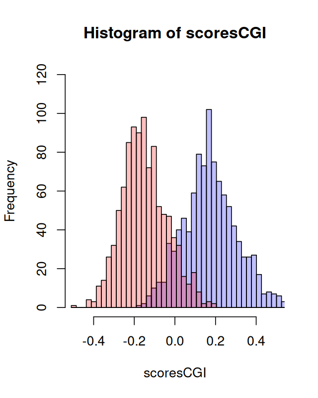

Figure 2.27: Island and non-island scores as generated by the function generateRandomScores. This is the first instance of a mixture we encounter. We will revisit them in Chapter 4.

We can consider these our training data: from data for which we know the types, we can see whether our score is useful for discriminating – see Figure 2.27.

2.11 Summary of this chapter

In this chapter we experienced the basic yoga of statistics: how to go from the data back to the possible generating distributions and how to estimate the parameters that define these distributions.

Statistical models We showed some specific statistical models for experiments with categorical outcomes (binomial and multinomial).

Goodness of fit We used different visualizations and showed how to run simulation experiments to test whether our data could be fit by a fair four box multinomial model. We encountered the chi-square statistic and saw how to compare simulation and theory using a qq-plot.

Estimation We explained maximum likelihood and Bayesian estimation procedures. These approaches were illustrated on examples involving nucleotide pattern discovery and haplotype estimations.

Prior and posterior distributions When assessing data of a type that has been been previously studied, such as haplotypes, it can be beneficial to compute the posterior distribution of the data. This enables us to incorporate uncertainty in the decision making, by way of a simple computation. The choice of the prior has little effect on the result as long as there is sufficient data.

CpG islands and Markov chains We saw how dependencies along DNA sequences can be modeled by Markov chain transitions. We used this to build scores based on likelihood ratios that enable us to see whether long DNA sequences come from CpG islands or not. When we made the histogram of scores, we saw in Figure 2.27 a noticeable feature: it seemed to be made of two pieces. This bimodality was our first encounter with mixtures, they are the subject of Chapter 4.

This is the first instance of building a model on some training data: sequences which we knew were in CpG islands, that we could use later to classify new data. We will develop a much more complete way of doing this in Chapter 12.

2.12 Further reading

One of the best introductory statistics books available is Freedman, Pisani, and Purves (1997). It uses box models to explain the important concepts. If you have never taken a statistics class, or you feel you need a refresher, we highly recommend it. Many introductory statistics classes do not cover statistics for discrete data in any depth. The subject is an important part of what we need for biological applications. A book-long introduction to these types of analyses can be found in (Agresti 2007).

Here we gave examples of simple unstructured multinomials. However, sometimes the categories (or boxes) of a multinomial have specific structure. For instance, the 64 possible codons code for 20 amino acids and the stop codons (61+3). So we can see the amino acids themselves as a multinomial with 20 degrees of freedom. Within each amino acid there are multinomials with differing numbers of categories (Proline has four: CCA, CCG, CCC, CCT, see Exercise 2.3). Some multivariate methods have been specifically designed to decompose the variability between codon usage within the differently abundant amino-acids (Grantham et al. 1981; Perrière and Thioulouse 2002), and this enables discovery of latent gene transfer and translational selection. We will cover the specific methods used in those papers when we delve into the multivariate exploration of categorical data in Chapter 9.

There are many examples of successful uses of the Bayesian paradigm to quantify uncertainties. In recent years the computation of the posterior distribution has been revolutionized by special types of Monte Carlo that use either a Markov chain or random walk or Hamiltonian dynamics. These methods provide approximations that converge to the correct posterior distribution after quite a few iterations. For examples and much more see (Robert and Casella 2009; Marin and Robert 2007; McElreath 2015).

2.13 Exercises

Exercise 2.1

Generate 1,000 random 0/1 variables that model mutations occurring along a 1,000 long gene sequence. These occur independently at a rate of \(10^{-4}\) each. Then sum the 1,000 positions to count how many mutations in sequences of length 1,000.

Find the correct distribution for these mutation sums using a goodness of fit test and make a plot to visualize the quality of the fit.

Exercise 2.2

Make a function that generates \(n\) random uniform numbers between \(0\) and \(7\) and returns their maximum. Execute the function for \(n=25\). Repeat this procedure \(B=100\) times. Plot the distribution of these maxima.
What is the maximum likelihood estimate of the maximum of a sample of size 25 (call it \(\hat{\theta}\))?
Can you find a theoretical justification and the true maximum \(\theta\)?

Exercise 2.3

A sequence of three nucleotides (a codon) taken in a coding region of a gene can be transcribed into one of 20 possible amino acids. There are \(4^3=64\) possible codon sequences, but only 20 amino acids. We say the genetic code is redundant: there are several ways to spell each amino acid.

The multiplicity (the number of codons that code for the same amino acid) varies from 2 to 6. The different codon-spellings of each amino acid do not occur with equal probabilities. Let’s look at the data for the standard laboratory strain of tuberculosis (H37Rv):

mtb = read.table("../data/M_tuberculosis.txt", header = TRUE)
head(mtb, n = 4)

  AmAcid Codon Number PerThous
1    Gly   GGG  25874    19.25
2    Gly   GGA  13306     9.90
3    Gly   GGT  25320    18.84
4    Gly   GGC  68310    50.82

The codons for the amino acid proline are of the form \(CC*\), and they occur with the following frequencies in Mycobacterium turberculosis:

pro  =  mtb[ mtb$AmAcid == "Pro", "Number"]
pro/sum(pro)

[1] 0.54302025 0.10532985 0.05859765 0.29305225

1. Explore the data mtb using table to tabulate the AmAcid and Codon variables.

2. How was the PerThous variable created?

3. Write an R function that you can apply to the table to find which of the amino acids shows the strongest codon bias, i.e., the strongest departure from uniform distribution among its possible spellings.

\(*\) stands for any of the 4 letters, using the computer notation for a regular expression.

Exercise 2.4

Display GC content in a running window along the sequence of Staphylococcus Aureus. Read in a fasta file sequence from a file.

staph = readDNAStringSet("../data/staphsequence.ffn.txt", "fasta")

1. Look at the complete staph object and then display the first three sequences in the set.

2. Find the GC content along the sequence in sliding windows of width 100.

3. Display the result of b).

4. How could we visualize the overall trends of these proportions along the sequence?

Solution

1. The data is displayed using:

staph[1:3, ]

DNAStringSet object of length 3:
    width seq                                               names               
[1]  1362 ATGTCGGAAAAAGAAATTTGGGA...AAAAAGAAATAAGAAATGTATAA lcl|NC_002952.2_c...
[2]  1134 ATGATGGAATTCACTATTAAAAG...TTTTACCAATCAGAACTTACTAA lcl|NC_002952.2_c...
[3]   246 GTGATTATTTTGGTTCAAGAAGT...TCATTCATCAAGGTGAACAATGA lcl|NC_002952.2_c...

staph

DNAStringSet object of length 2650:
       width seq                                            names               
   [1]  1362 ATGTCGGAAAAAGAAATTTGGG...AAAGAAATAAGAAATGTATAA lcl|NC_002952.2_c...
   [2]  1134 ATGATGGAATTCACTATTAAAA...TTACCAATCAGAACTTACTAA lcl|NC_002952.2_c...
   [3]   246 GTGATTATTTTGGTTCAAGAAG...ATTCATCAAGGTGAACAATGA lcl|NC_002952.2_c...
   [4]  1113 ATGAAGTTAAATACACTCCAAT...CAAGGTGAAATTATAAAGTAA lcl|NC_002952.2_c...
   [5]  1932 GTGACTGCATTGTCAGATGTAA...TATGCAAACTTAGACTTCTAA lcl|NC_002952.2_c...
   ...   ... ...
[2646]   720 ATGACTGTAGAATGGTTAGCAG...ACTCCTTTACTTGAAAAATAA lcl|NC_002952.2_c...
[2647]  1878 GTGGTTCAAGAATATGATGTAA...CTCCAAAGGGTGAGTGACTAA lcl|NC_002952.2_c...
[2648]  1380 ATGGATTTAGATACAATTACGA...CAATTCTGCTTAGGTAAATAG lcl|NC_002952.2_c...
[2649]   348 TTGGAAAAAGCTTACCGAATTA...TTTAATAAAAAGATTAAGTAA lcl|NC_002952.2_c...
[2650]   138 ATGGTAAAACGTACTTATCAAC...CGTAAAGTTTTATCTGCATAA lcl|NC_002952.2_c...

2. We can compute the frequencies using the function letterFrequency.

letterFrequency(staph[[1]], letters = "ACGT", OR = 0)

  A   C   G   T 
522 219 229 392 

GCstaph = data.frame(
  ID = names(staph),
  GC = rowSums(alphabetFrequency(staph)[, 2:3] / width(staph)) * 100
)

3. Plotting can be done as follows, here exemplarily for sequence 364 (Figure 2.28):

window = 100
gc = rowSums( letterFrequencyInSlidingView(staph[[364]], window,
      c("G","C")))/window
plot(x = seq(along = gc), y = gc, type = "l")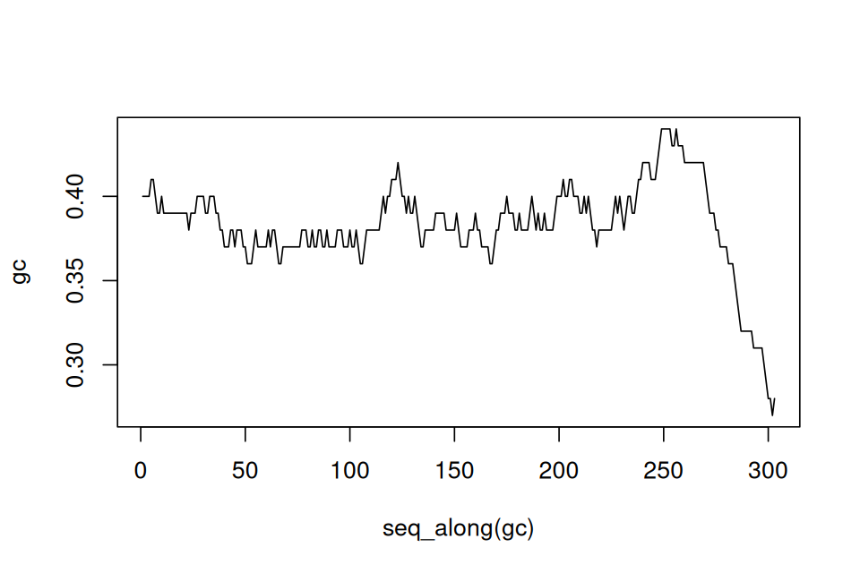

Figure 2.28: GC content along sequence 364 of the Staphylococcus Aureus genome.

4. We can look at the overall trends by smoothing the data using the function lowess along a window.

plot(x = seq(along = gc), y = gc, type = "l")
lines(lowess(x = seq(along = gc), y = gc, f = 0.2), col = 2)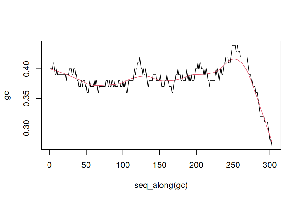

Figure 2.29: Similar to Figure 2.28, with smoothing.

We will see later an appropriate way of deciding whether the window has an abnormally high GC content by using the idea that as we move along the sequences, we are always in one of several possible states. However, we don’t directly observe the state, just the sequence. Such models are called hidden (state) Markov models, or HMM for short (see Wikipedia). The Markov in the name of these models is for how they model dependencies between neighboring positions, the hidden part indicates that the state is not directly observed, that is, hidden.

Exercise 2.5

Redo a figure similar to Figure 2.19, but include two other distributions: the uniform (which is Beta(1,1)) and Beta(\(\frac{1}{2},\frac{1}{2}\)). What do you notice?

Solution

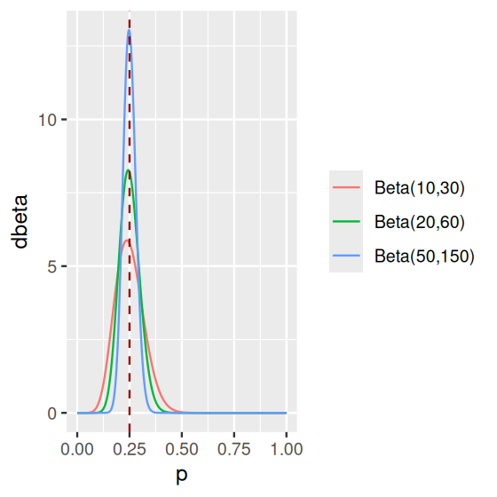
dfbetas = data.frame(
  p = rep(p_seq, 5),
  dbeta = c(dbeta(p_seq, 0.5, 0.5), 
            dbeta(p_seq,   1,   1), 
            dbeta(p_seq,  10,  30),
            dbeta(p_seq,  20,  60), 
            dbeta(p_seq,  50, 150)),
  pars = rep(c("Beta(0.5,0.5)", "U(0,1)=Beta(1,1)", 
               "Beta(10,30)", "Beta(20,60)", 
               "Beta(50,150)"), each = length(p_seq)))
ggplot(dfbetas) +
  geom_line(aes(x = p, y = dbeta, colour = pars)) +
  theme(legend.title = element_blank()) +
  geom_vline(aes(xintercept = 0.25), colour = "#990000", linetype = "dashed")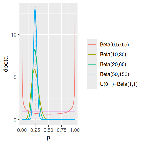

Figure 2.30: Beta densities for different parameter choices.

Whereas the Beta distributions with parameters larger than one are unimodal, the Beta(0.5,0.5) distribution is bimodal and the Beta(1,1) is flat and has no mode.

Exercise 2.6

Choose your own prior for the parameters of the Beta distribution. You can do this by sketching it here: https://jhubiostatistics.shinyapps.io/drawyourprior. Once you have set up a prior, re-analyse the data from Section 2.9.1, where we saw \(Y = 40\) successes out of \(n=300\) trials. Compare your posterior distribution to the one we obtained in that section using a QQ-plot.

Agresti, Alan. 2007. An Introduction to Categorical Data Analysis. John Wiley.

Cannings, Chris, and Anthony WF Edwards. 1968. “Natural Selection and the de Finetti Diagram.” Annals of Human Genetics 31 (4): 421–28.

Cleveland, William S. 1988. The Collected Works of John w. Tukey: Graphics 1965-1985. Vol. 5. CRC Press.

Durbin, Richard, Sean Eddy, Anders Krogh, and Graeme Mitchison. 1998. Biological Sequence Analysis. Cambridge University Press.

Elson, D, and E Chargaff. 1952. “On the Desoxyribonucleic Acid Content of Sea Urchin Gametes.” Experientia 8 (4): 143–45.

Finetti, Bruno de. 1926. “Considerazioni Matematiche Sull’ereditarieta Mendeliana.” Metron 6: 3–41.

Freedman, David, Robert Pisani, and Roger Purves. 1997. Statistics. New York, NY: WW Norton.

Grantham, Richard, Christian Gautier, Manolo Gouy, M Jacobzone, and R Mercier. 1981. “Codon Catalog Usage Is a Genome Strategy Modulated for Gene Expressivity.” Nucleic Acids Research 9 (1): 213–13.

Irizarry, Rafael A, Hao Wu, and Andrew P Feinberg. 2009. “A Species-Generalized Probabilistic Model-Based Definition of CpG Islands.” Mammalian Genome 20 (9-10): 674–80.

Love, Michael I, Wolfgang Huber, and Simon Anders. 2014. “Moderated Estimation of Fold Change and Dispersion for RNA-seq Data with DESeq2.” Gnome Biology 15 (12): 1–21.

Marin, Jean-Michel, and Christian Robert. 2007. Bayesian Core: A Practical Approach to Computational Bayesian Statistics. Springer Science & Business Media.

McElreath, Richard. 2015. Statistical Rethinking: A Bayesian Course with Examples in R and Stan. Chapman; Hall/CRC.

Mourant, AE, Ada Kopec, and K Domaniewska-Sobczak. 1976. “The Distribution of the Human Blood Groups 2nd Edition.” Oxford University Press London.

Perrière, Guy, and Jean Thioulouse. 2002. “Use and Misuse of Correspondence Analysis in Codon Usage Studies.” Nucleic Acids Research 30 (20): 4548–55.

Rice, John. 2006. Mathematical Statistics and Data Analysis. Cengage Learning.

Robert, Christian, and George Casella. 2009. Introducing Monte Carlo Methods with R. Springer Science & Business Media.

Page built at 21:12 on 2024-04-15 using R version 4.3.3 (2024-02-29)