4 Mixture Models

One of the main challenges of biological data analysis is dealing with heterogeneity. The quantities we are interested in often do not show a simple, unimodal “textbook distribution”. For example, in the last part of Chapter 2 we saw how the histogram of sequence scores in Figure 2.27 had two separate modes, one for CpG-islands and one for non-islands. We can see the data as a simple mixture of a few (in this case: two) components. We call these finite mixtures. Other mixtures can involve almost as many components as we have observations. These we call infinite mixtures¹.

¹ We will see that—as for so many modeling choices–the right complexity of the mixture is in the eye of the beholder and often depends on the amount of data and the resolution and smoothness we want to attain.

In Chapter 1 we saw how a simple generative model with a Poisson distribution led us to make useful inference in the detection of an epitope. Unfortunately, a satisfactory fit to real data with such a simple model is often out of reach. However, simple models such as the normal or Poisson distributions can serve as building blocks for more realistic models using the mixing framework that we cover in this chapter. Mixtures occur naturally for flow cytometry data, biometric measurements, RNA-Seq, ChIP-Seq, microbiome and many other types of data collected using modern biotechnologies. In this chapter we will learn from simple examples how to build more realistic models of distributions using mixtures.

4.1 Goals for this chapter

In this chapter we will:

Generate our own mixture model data from distributions composed of two normal populations.
See how the Expectation-Maximization (EM) algorithm enables us to “reverse engineer” the underlying mixtures in dataset.
Use a special type of mixture called zero-inflation for data such as ChIP-Seq data that have many extra zeros.
Discover the empirical cumulative distribution: a special mixture that we can build from observed data. This will enable us to see how we can simulate the variability of our estimates using the bootstrap.
Build the Laplace distribution as an instance of an infinite mixture model with many components. We will use it to model promoter lengths and microarray intensities.
Have our first encounter with the gamma-Poisson distribution, a hierarchical model useful for RNA-Seq data. We will see it comes naturally from mixing different Poisson distributed sources.
See how mixture models enable us to choose data transformations.

4.2 Finite mixtures

4.2.1 Simple examples and computer experiments

Here is a first example of a mixture model with two equal-sized components. The generating process has two steps:

Flip a fair coin.

If it comes up heads: Generate a random number from a normal distribution with mean 1 and variance 0.25.

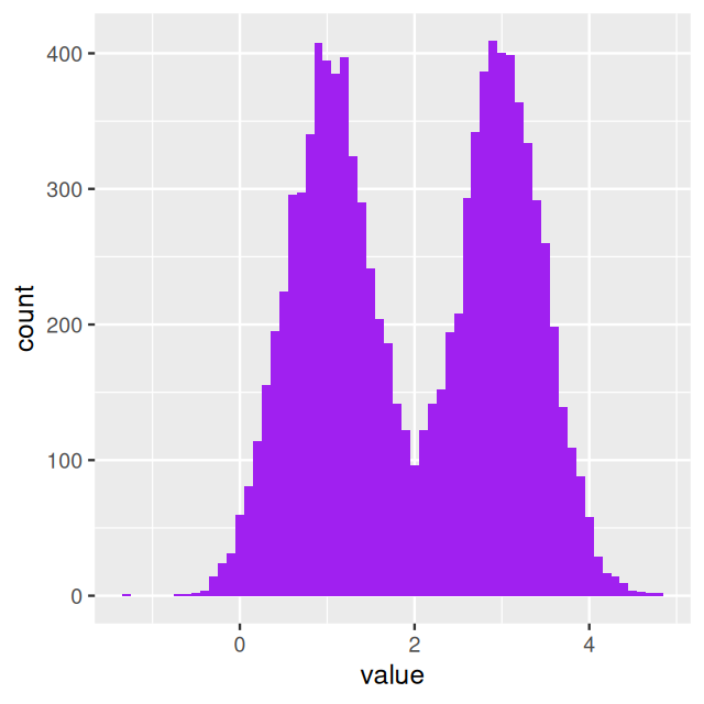
If it comes up tails: Generate a random number from a normal distribution with mean 3 and variance 0.25. The histogram shown in Figure 4.1 was produced by repeating these two steps 10000 times using the following code.

coinflips = (runif(10000) > 0.5)
table(coinflips)

coinflips
FALSE  TRUE 
 5016  4984

oneFlip = function(fl, mean1 = 1, mean2 = 3, sd1 = 0.5, sd2 = 0.5) {
  if (fl) {
   rnorm(1, mean1, sd1)
  } else {
   rnorm(1, mean2, sd2)
  }
}
fairmix = vapply(coinflips, oneFlip, numeric(1))
library("ggplot2")
library("dplyr")
ggplot(tibble(value = fairmix), aes(x = value)) +
     geom_histogram(fill = "purple", binwidth = 0.1)

Figure 4.1: Histogram of 10,000 random draws from a fair mixture of two normals. The left hand part of the histogram is dominated by numbers generated from (A), on the right from (B).

Question 4.1

How can you use R’s vectorized syntax to remove the vapply-loop and generate the fairmix vector more efficiently?

Solution

means = c(1, 3)
sds   = c(0.5, 0.5)
values = rnorm(length(coinflips),
               mean = ifelse(coinflips, means[1], means[2]),
               sd   = ifelse(coinflips, sds[1],   sds[2]))

Question 4.2

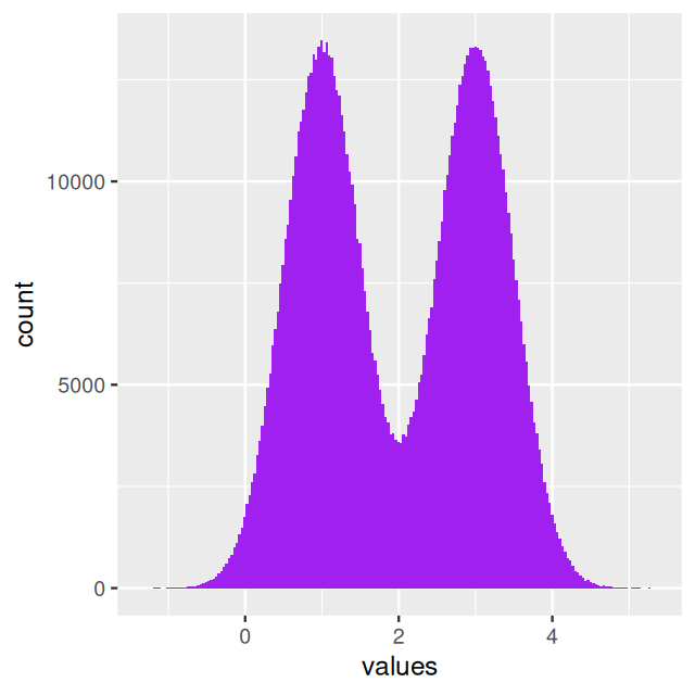
Using your improved code, use one million coin flips and make a histogram with 200 bins. What do you notice?

Solution

fair = tibble(
  coinflips = (runif(1e6) > 0.5),
  values = rnorm(length(coinflips),
                 mean = ifelse(coinflips, means[1], means[2]),
                 sd   = ifelse(coinflips, sds[1],   sds[2])))
ggplot(fair, aes(x = values)) +
     geom_histogram(fill = "purple", bins = 200)

Figure 4.2: Similar to Figure 4.1, but with one million observations.

Figure 4.2 illustrates that as we increase the number of bins and the number of observations per bin, the histogram approaches a smooth curve. This smooth limiting curve is called the density function of the random variable fair$values.

The density function for a normal $N(\mu,\sigma)$ random variable can be written explicitly. We usually call it

\[ \phi(x)=\frac{1}{\sigma \sqrt{2\pi}}e^{-\frac{1}{2}(\frac{x-\mu}{\sigma})^2}. \]

Question 4.3

Plot a histogram of those values of fair$values for which coinflips is TRUE. Hint: use y = ..density.. in the call to aes (which means that the vertical axis is to show the proportion of counts) and set the binwidth to 0.01.
Overlay the line corresponding to $\phi(z)$.

Solution

ggplot(dplyr::filter(fair, coinflips), aes(x = values)) +
  geom_histogram(aes(y = after_stat(density)), fill = "purple", binwidth = 0.01) +
  stat_function(fun = dnorm, color = "red",
                args = list(mean = means[1], sd = sds[1]))

Figure 4.3: Histogram of half a million draws from the normal distribution $N(\mu=1,\sigma^2=0.5^2)$. The curve is the theoretical density $\phi(x)$ calculated using the function `dnorm`.

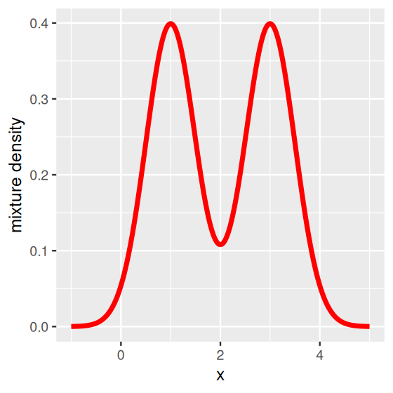
In fact we can write the mathematical formula for the density of all of fair$values (the limiting curve that the histograms tend to look like) as a sum of the two densities.

\[ f(x)=\frac{1}{2}\phi_1(x)+\frac{1}{2}\phi_2(x), \tag{4.1}\]

where $\phi_1$ is the density of the normal $N(\mu_1=1,\sigma^2=0.25)$ and $\phi_2$ is the density of the normal $N(\mu_2=3,\sigma^2=0.25)$. Figure 4.4 was generated by the following code.

fairtheory = tibble(
  x = seq(-1, 5, length.out = 1000),
  f = 0.5 * dnorm(x, mean = means[1], sd = sds[1]) +
      0.5 * dnorm(x, mean = means[2], sd = sds[2]))
ggplot(fairtheory, aes(x = x, y = f)) +
  geom_line(color = "red", linewidth = 1.5) + ylab("mixture density")

Figure 4.4: The theoretical density of the mixture.

In this case, the mixture model is extremely visible as the two component distributions have little overlap. Figure 4.4 shows two distinct peaks: we call this a bimodal distribution. In practice, in many cases the separation between the mixture components is not so obvious—but nevertheless relevant.

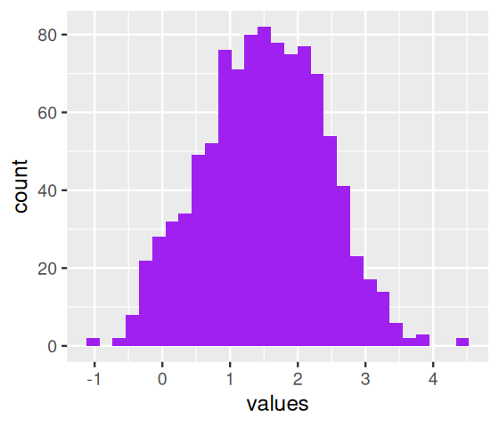
Figure 4.5: A mixture of two normals that is harder to recognize.

Question 4.4

Figure 4.5 is a histogram of a fair mixture of two normals with the same variances. Can you guess the two mean parameters of the component distributions? Hint: you can use trial and error, and simulate various mixtures to see if you can make a matching histogram. Looking at the R code for the chapter will show you exactly how the data were generated.

Solution

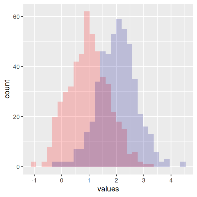
The following code colors in red the points that were generated from the heads coin flips and in blue those from the tails. Its output, in Figure 4.6, shows the two underlying distributions.

head(mystery, 3)

# A tibble: 3 × 2
  coinflips values
  <lgl>      <dbl>
1 FALSE      1.64 
2 TRUE       0.607
3 FALSE      1.77

br = with(mystery, seq(min(values), max(values), length.out = 30))
ggplot(mystery, aes(x = values)) +
  geom_histogram(data = dplyr::filter(mystery, coinflips),
     fill = "red", alpha = 0.2, breaks = br) +
  geom_histogram(data = dplyr::filter(mystery, !coinflips),
     fill = "darkblue", alpha = 0.2, breaks = br)

Figure 4.6: The mixture from Figure 4.5, but with the two components colored in red and blue.

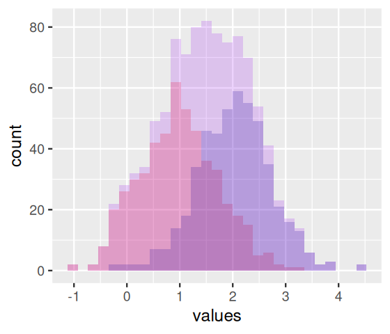
In Figure 4.6, the bars from the two component distributions are plotted on top of each other. A different way of showing the components is Figure 4.7, produced by the code below.

ggplot(mystery, aes(x = values, fill = coinflips)) +
  geom_histogram(data = dplyr::filter(mystery, coinflips),
     fill = "red", alpha = 0.2, breaks = br) +
  geom_histogram(data = dplyr::filter(mystery, !coinflips),
     fill = "darkblue", alpha = 0.2, breaks = br) +
  geom_histogram(fill = "purple", breaks = br, alpha = 0.2)

Figure 4.7: As Figure 4.6, with stacked bars for the two mixture components.

Question 4.5

Why do the bars in Figure 4.7, but not those in Figure 4.6 have the same heights as in Figure 4.5?

Solution

In Figures 4.7 and 4.5, each count occupies a different piece of vertical space in a bin. In Figure 4.6, in the overlapping (darker) region, some of the counts falling within the same bin are overplotted.

In Figures 4.6 and 4.7, we were able to use the coinflips column in the data to disentangle the components. In real data, this information is missing.

4.2.2 Discovering the hidden class labels

We use a method called the expectation-maximization (EM) algorithm to infer the value of the hidden groupings. The EM algorithm is a popular iterative procedure that alternates between pretending we know one part of the solution to compute the other part, and pretending the other part is known and computing the first part, and so on, until convergence. More concretely, it alternates between

pretending we know the probabilities with which each observation belongs to the different mixture components and, from this, estimating the parameters of the components, and
pretending we know the parameters of the mixture components and estimating the probabilities with which each observation belongs to the components.

Let’s take a simple example. We measure a variable $x$ on a series of objects that we think come from two groups, although we do not know the group labels. We start by augmenting² the data with the unobserved (latent) group label, which we will call $U$.

² Adding another variable which was not measured, called a hidden or latent variable.

We are interested in finding the values of $U$ and the unknown parameters $\theta$ of the underlying distribution of the groups. We will use the maximum likelihood approach introduced in Chapter 2 to estimate the parameters that make the data $x$ the most likely. We can write the probability densities

\[ p(x,u\,|\,\theta) = p(x\,|\,u,\theta)\,p(u\,|\,\theta). \tag{4.2}\]

Mixture of normals

For instance, we could generalize our previous mixture model with two normal distributions Equation 4.1 by allowing non-equal mixture fractions,

\[ f(x)=\lambda\phi_1(x)+(1-\lambda)\phi_2(x), \tag{4.3}\]

for $\lambda\in[0,1]$. Similarly as above, $\phi_k$ is the density of the normal $N(\mu_k,\sigma_k^2)$ for $k=1$ and $k=2$, respectively. Then, the parameter vector $\theta$ is a five-tuple of the two means, the two standard deviations, and the mixture parameter $\lambda$. In other words, $\theta=(\mu_1,\mu_2,\sigma_1,\sigma_2,\lambda)$. Here is an example of data generated according to such a model. The labels are denoted by $u$.

mus = c(-0.5, 1.5)
lambda = 0.5
u = sample(2, size = 100, replace = TRUE, prob = c(lambda, 1-lambda))
x = rnorm(length(u), mean = mus[u])
dux = tibble(u, x)
head(dux)

# A tibble: 6 × 2
      u      x
  <int>  <dbl>
1     2  0.731
2     1 -1.25 
3     2  3.07 
4     1 -0.333
5     2  2.64 
6     1  0.314

If we know the labels $u$, we can estimate the parameters using separate MLEs for each group. The overall likelihood is

\[ p(x, u \,|\, \theta) = \left( \prod_{\{i:\,u_i=1\}} \phi_1(x_i) \right) \times \left( \prod_{\{i:\,u_i=2\}} \phi_2(x_i) \right). \tag{4.4}\]

Its maximization can be split into three independent pieces: we find $\mu_1$ and $\sigma_1$ by maximizing the first bracketed expression on the right hand side of Equation 4.4, $\mu_2$ and $\sigma_2$ by maximizing the second, and $\lambda$ from the empirical frequencies of the labels:

group_by(dux, u) |> summarize(mu = mean(x), sigma = sd(x))

# A tibble: 2 × 3
      u     mu sigma
  <int>  <dbl> <dbl>
1     1 -0.684 1.13 
2     2  1.64  0.996

table(dux$u) / nrow(dux)


   1    2 
0.49 0.51

Question 4.6

Suppose we knew the mixing proportion $\lambda=\frac{1}{2}$, but not the $u_i$, so that the density is $\frac{1}{2}\phi_1(x)+\frac{1}{2}\phi_2(x)$. Try writing out the (log) likelihood. What prevents us from solving for the MLE explicitly here?

Solution

See, e.g., the chapter on Mixture Models in Shalizi (2017) for the computation of the likelihood of a finite mixture of normals. “If we try to estimate the mixture model, then, we’re doing weighted maximum likelihood, with weights given by the posterior label probabilities. These, to repeat, depend on the parameters we are trying to estimate, so there seems to be a vicious circle.”

In many cases we neither know the $u$ labels nor the mixture proportions. What we can do is start with an initial guess for the labels and pretend to know them, estimate the parameters as above, and then go through an iterative cycle, updating at each step our current best guess of the labels and the parameters until our estimates no longer substantially change (i.e., until they seem to have converged) and the likelihood has reached an optimum.

In fact we can do something more elaborate and replace the “hard” labels $u$ for each observation (it is either in group 1 or 2) by membership weights that sum up to 1. The mixture model 4.3 suggests that we interpret

\[ w(x, 1) = \frac{\lambda\phi_1(x)}{\lambda\phi_1(x)+(1-\lambda)\phi_2(x)} \tag{4.5}\]

as the probability that an observation with value $x$ was generated by the first mixture component, and analogously $w(x, 2) = 1 - w(x, 1)$ for the second component. In other words, while $\lambda$ is the prior probability that an observation that we have not yet seen comes from mixture component 1, $w(x,1)$ is the corresponding posterior probability once we have observed its value $x$. This suggests the following iterative algorithm:

E step: Assuming that $\theta$ (i.e., the means, standard deviations and $\lambda$) is known, evaluate the membership weights 4.5.

M step: Given the membership weights of each observation $x_i$, determine a new, improved maximum likelihood estimate of $\theta$.

Iterate until $\theta$ and the likelihood have converged. At this point, please check out Exercise 4.1 for a worked out demonstration with code. In fact, this algorithm is far more general than our particular application example here. A very readable exposition is presented by (Bishop 2006), here some of the highlights:

Our goal is to maximize the marginal likelihood of a probabilistic model that involves an observed variable $x$, an unobserved variable $u$ and some parameter $\theta$. In our simple example, $u$ is a categorical variable with two possible values, and $x$ a real number. In general, both $x$ and $u$ can be a tuple of multiple individual variables (i.e., they can be multivariate) of any variable type. The marginal likelihood is computed by taking the expectation (i.e., a weighted average) across all possible values of $u$:

\[ L_\text{marg}(\theta; x) = \int_U p(x, u\,|\,\theta) \, \text{d}U. \tag{4.6}\]

In our specific example, the integration amounts to (probabilistically) averaging over all possible membership configurations, and thus, to the weighted sum taking into account the membership weights,

\[ L_\text{marg}(\theta; x) = \prod_{i=1}^n \sum_{u=1}^2 p(x_i, u\,|\,\theta) \, w(x_i, u\,|\,\theta). \tag{4.7}\]

Directly maximizing this quantity is intractable.

Something we do have a grip on, given the data and our current parameter estimate $\theta_t$, is the conditional distribution of the latent variable, $p(u\,|\,x, \theta_t)$. We can use it to find the expectation of the complete data log likelihood $\log p(x, u\,|\,\theta)$ evaluated for some general parameter value $\theta$. This expectation is often denoted as

\[ Q(\theta, \theta_t) = \int_U \log p(x, u\,|\,\theta) \, p(u\,|\, x, \theta_t) \, \text{d}U. \tag{4.8}\]

In the M step, we determine the revised parameter estimate $\theta_{t+1}$ by maximizing this function,

\[ \theta_{t+1} = \arg \max_\theta \, Q(\theta, \theta_t). \tag{4.9}\]

The E step consists of computing $p(u\,|\, x, \theta_t)$, the essential ingredient of $Q$.

These two steps (E and M) are iterated until the improvements are small; this is a numerical indication that we are close to a flattening of the likelihood and have reached a maximum. The iteration trajectory, but hopefully not the point that we arrive at, will depend on the starting point. This is analogous to a hike to the top of a mountain, which can start at different places and may take different routes, but always leads to the top of the hill—as long as there is only one hilltop and not several. Thus, as a precaution, it is good practice to repeat such a procedure several times from different starting points and make sure that we always get the same answer.

Question 4.7

Several R packages provide EM implementations, including mclust, EMcluster and EMMIXskew. Choose one and run the EM function several times with different starting values. Then use the function normalmixEM from the mixtools package to compare the outputs.

Solution

Here we show the output from mixtools.

library("mixtools")
y = c(rnorm(100, mean = -0.2, sd = 0.5),
      rnorm( 50, mean =  0.5, sd =   1))
gm = normalmixEM(y, k = 2, 
                    lambda = c(0.5, 0.5),
                    mu = c(-0.01, 0.01), 
                    sigma = c(3, 3))

number of iterations= 169

with(gm, c(lambda, mu, sigma, loglik))

[1]    0.4482    0.5518   -0.2268    0.0802    0.3941    0.9370 -166.1471

The EM algorithm is very instructive:

We saw a first example of soft averaging, where we don’t decide whether an observation belongs to one group or another, but allow it to participate in several groups by using membership probabilities as weights, and thus obtain more nuanced estimates (Slonim et al. 2005).
It shows us how we can tackle a difficult problem with too many unknowns by alternating between solving simpler problems.
We were able to consider a data generating model with hidden variables, and still estimate its parameters. We could do so even without explicitly commiting on the values of the hidden variables: we took a (weighted) average over them, in the Expecation step of Equation 4.8, embodied by the membership probabilities. This basic idea is so powerful that it is the starting point for many more advanced algorithms in machine learning (Bishop 2006).
It can be extended to the more general case of model averaging (Hoeting et al. 1999). It can be sometimes beneficial to consider several models simultaneously if we are unsure which one is relevant for our data. We can combine them together into a weighted model. The weights are provided by the likelihoods of the models.

4.2.3 Models for zero inflated data

Ecological and molecular data often come in the form of counts. For instance, this may be the number of individuals from each of several species at each of several locations. Such data can often be seen as a mixture of two scenarios: if the species is not present, the count is necessarily zero, but if the species is present, the number of individuals we observe varies, with a random sampling distribution; this distribution may also include zeros. We model this as a mixture:

\[ f_{\text{zi}}(x) = \lambda \, \delta(x) + (1-\lambda) \, f_{\text{count}}(x), \tag{4.10}\]

where $\delta$ is Dirac’s delta function, which represents a probability distribution that has all its mass at 0. The zeros from the first mixture component are called “structural”: in our example, they occur because certain species do not live in certain habitats. The second component, $f_{\text{count}}$ may also include zeros and other small numbers, simply due to random sampling. The R packages pscl (Zeileis, Kleiber, and Jackman 2008) and zicounts provide many examples and functions for working with zero inflated counts.

Example: ChIP-Seq data

Let’s consider the example of ChIP-Seq data. These data are sequences of pieces of DNA that are obtained from chromatin immunoprecipitation (ChIP). This technology enables the mapping of the locations along genomic DNA of transcription factors, nucleosomes, histone modifications, chromatin remodeling enzymes, chaperones, polymerases and other protein. It was the main technology used by the Encyclopedia of DNA Elements (ENCODE) Project. Here we use an example (Kuan et al. 2011) from the mosaicsExample package, which shows data measured on chromosome 22 from ChIP-Seq of antibodies for the STAT1 protein and the H3K4me3 histone modification applied to the GM12878 cell line. Here we do not show the code to construct the binTFBS object; it is shown in the source code file for this chapter and follows the vignette of the mosaics package.

binTFBS

Summary: bin-level data (class: BinData)
----------------------------------------
- # of chromosomes in the data: 1
- total effective tag counts: 462479
  (sum of ChIP tag counts of all bins)
- control sample is incorporated
- mappability score is NOT incorporated
- GC content score is NOT incorporated
- uni-reads are assumed
----------------------------------------

From this object, we can create the histogram of per-bin counts.

bincts = print(binTFBS)
ggplot(bincts, aes(x = tagCount)) +
  geom_histogram(binwidth = 1, fill = "forestgreen")

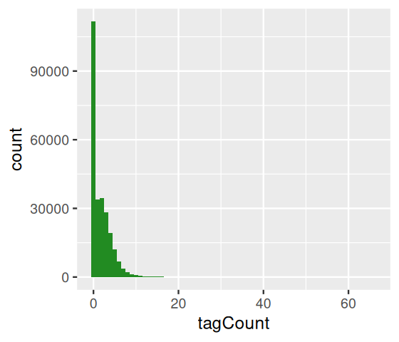
Figure 4.8: The number of binding sites found in 200nt windows along chromosome 22 in a ChIP-Seq dataset.

We see in Figure 4.8 that there are many zeros, although from this plot it is not immediately obvious whether the number of zeros is really extraordinary, given the frequencies of the other small numbers ($1,2,...$).

Question 4.8

Redo the histogram of the counts using a logarithm base 10 scale on the $y$-axis.
Estimate $\pi_0$, the proportion of bins with zero counts.

Solution

ggplot(bincts, aes(x = tagCount)) + scale_y_log10() +
   geom_histogram(binwidth = 1, fill = "forestgreen")

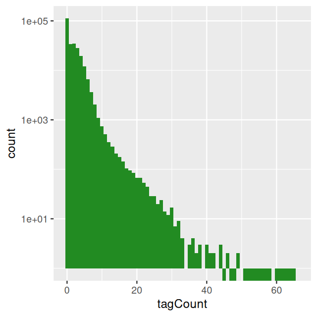
Figure 4.9: As Figure 4.8, but using a logarithm base 10 scale on the $y$-axis. The fraction of zeros seems elevated compared to that of ones, twos, …

4.2.4 More than two components

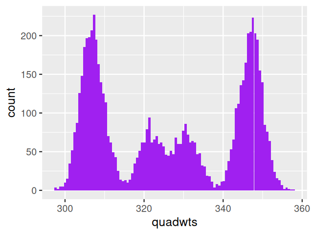
So far we have looked at mixtures of two components. We can extend our description to cases where there may be more. For instance, when weighing N=7,000 nucleotides obtained from mixtures of deoxyribonucleotide monophosphates (each type has a different weight, measured with the same standard deviation sd=3), we might observe the histogram (shown in Figure 4.10) generated by the following code.

masses = c(A =  331, C =  307, G =  347, T =  322)
probs  = c(A = 0.12, C = 0.38, G = 0.36, T = 0.14)
N  = 7000
sd = 3
nuclt   = sample(length(probs), N, replace = TRUE, prob = probs)
quadwts = rnorm(length(nuclt),
                mean = masses[nuclt],
                sd   = sd)
ggplot(tibble(quadwts = quadwts), aes(x = quadwts)) +
  geom_histogram(bins = 100, fill = "purple")

Figure 4.10: Simulation of 7,000 nucleotide mass measurements.

Question 4.9

Repeat this simulation experiment with $N=1000$ nucleotide measurements. What do you notice in the histogram?

Question 4.10

What happens when $N=7000$ but the standard deviation is 10?

Question 4.11

Plot the theoretical density curve for the distribution simulated in Figure 4.10.

In this case, as we have enough measurements with good enough precision, we are able to distinguish the four nucleotides and decompose the distribution shown in Figure 4.10. With fewer data and/or more noisy measurements, the four modes and the distribution component might be less clear.

4.3 Empirical distributions and the nonparametric bootstrap

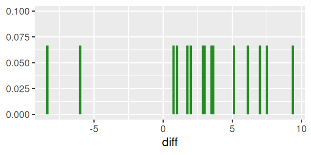
In this section, we will consider an extreme case of mixture models, where we model our sample of $n$ data points as a mixture of $n$ point masses. We could use almost any set of data here; to be concrete, we use Darwin’s Zea Mays data³ in which he compared the heights of 15 pairs of Zea Mays plants (15 self-hybridized versus 15 crossed). The data are available in the HistData package, and we plot the distribution of the 15 differences in height:

³ They were collected by Darwin who asked his cousin, Francis Galton to analyse them. R.A. Fisher re-analysed the same data using a paired t-test (Bulmer 2003). We will get back to this example in Chapter 13.

library("HistData")
ZeaMays$diff

 [1]  6.125 -8.375  1.000  2.000  0.750  2.875  3.500  5.125  1.750  3.625
[11]  7.000  3.000  9.375  7.500 -6.000

ggplot(ZeaMays, aes(x = diff, ymax = 1/15, ymin = 0)) +
  geom_linerange(linewidth = 1, col = "forestgreen") + ylim(0, 0.1)

Figure 4.11: The observed sample can be seen as a mixture of point masses at each of the values (real point masses would be bars without any width whatsoever).

In Section 3.6.7 we saw that the empirical cumulative distribution function (ECDF) for a sample of size $n$ is

\[ \hat{F}_n(x)= \frac{1}{n}\sum_{i=1}^n {\mathbb 1}_{x \leq x_i}, \tag{4.11}\]

and we saw ECDF plots in Figure 3.24. We can also write the density of our sample as

\[ \hat{f}_n(x) =\frac{1}{n}\sum_{i=1}^n \delta_{x_i}(x) \tag{4.12}\]

In general, the density of a probability distribution is the derivative (if it exists) of the distribution function. We have applied this principle here: the density of the distribution defined by Equation 4.11 is Equation 4.12. We could do this since one can consider the function $\delta_a$ the “derivative” of the step function ${\mathbb 1}_{x \leq a}$: it is completely flat almost everywhere, except at the one point $a$ where there is the step, and where its value is “infinite” . Equation 4.12 highlights that our data sample can be considered a mixture of $n$ point masses at the observed values $x_1,x_2,..., x_{n}$, such as in Figure 4.11.

There is a bit of advanced mathematics (beyond standard calculus) required for this to make sense, which is however beyond the scope of our treatment here.

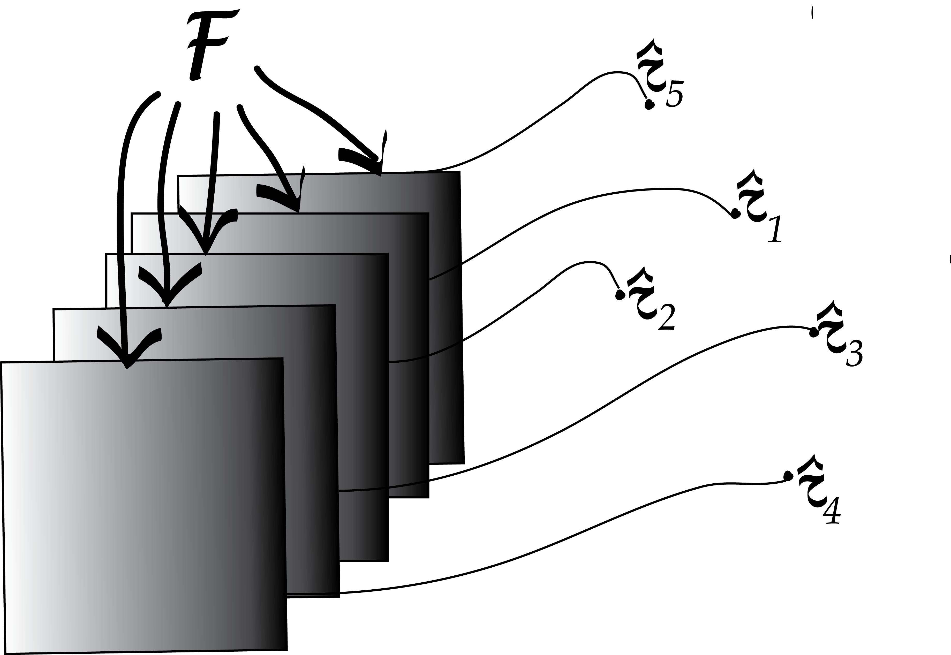
Figure 4.12: The value of a statistic $\tau$ is estimated from data (the grey matrices) generated from an underlying distribution $F$. Different samples from $F$ lead to different data, and so to different values of the estimate $\hat{\tau}$: this is called **sampling variability**. The distribution of all the $\hat{\tau}$’s is the **sampling distribution**.

Statistics of our sample, such as the mean, minimum or median, can now be written as a function of the ECDF, for instance, $\bar{x} = \int \delta_{x_i}(x)\,\text{d}x$. As another instance, if $n$ is an odd number, the median is $x_{(\frac{n+1}{2})}$, the value right in the middle of the ordered list.

The true sampling distribution of a statistic $\hat{\tau}$ is often hard to know as it requires many different data samples from which to compute the statistic; this is shown in Figure 4.12.

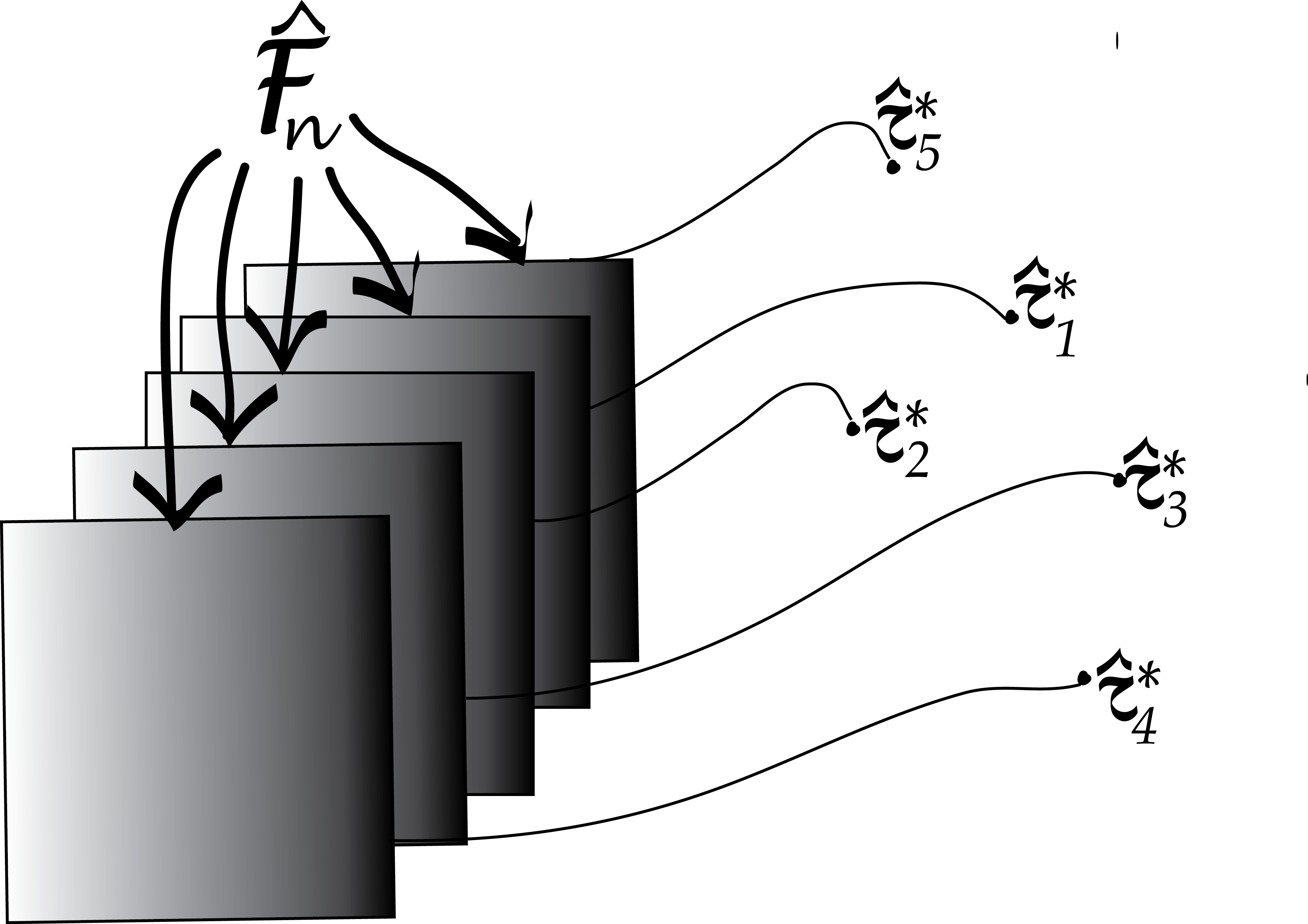
The bootstrap principle approximates the true sampling distribution of $\hat{\tau}$ by creating new samples drawn from the empirical distribution built from the original sample (Figure 4.13). We reuse the data (by considering it a mixture distribution of $\delta$s) to create new “datasets” by taking samples and looking at the sampling distribution of the statistics $\hat{\tau}^*$ computed on them. This is called the nonparametric bootstrap resampling approach, see Bradley Efron and Tibshirani (1994) for a complete reference. It is very versatile and powerful method that can be applied to basically any statistic, no matter how complicated it is. We will see example applications of this method, in particular to clustering, in Chapter 5.

Figure 4.13: The bootstrap simulates the sampling variability by drawing samples not from the underlying true distribution $F$ (as in Figure 4.12), but from the empirical distribution function $\hat{F}_n$.

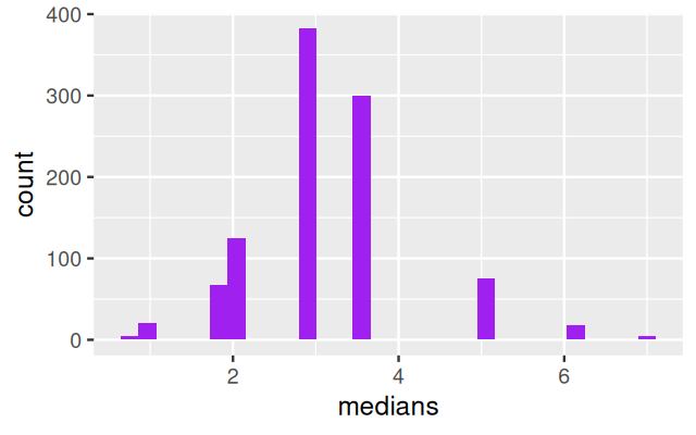
Using these ideas, let’s try to estimate the sampling distribution of the median of the Zea Mays differences we saw in Figure 4.11. We use similar simulations to those in the previous sections: Draw $B=1000$ samples of size 15 from the 15 values (each being a component in the 15-component mixture). Then compute the 1000 medians of each of these samples of 15 values and look at their distribution: this is the bootstrap sampling distribution of the median.

B = 1000
meds = replicate(B, {
  i = sample(15, 15, replace = TRUE)
  median(ZeaMays$diff[i])
})
ggplot(tibble(medians = meds), aes(x = medians)) +
  geom_histogram(bins = 30, fill = "purple")

Figure 4.14: The bootstrap sampling distribution of the median of the Zea Mays differences.

Question 4.12

Estimate a 99% confidence interval for the median based on these simulations. What can you conclude from looking at the overlap between this interval and 0?

Question 4.13

Use the bootstrap package to redo the same analysis using the function bootstrap for both median and mean. What differences do you notice between the sampling distribution of the mean and the median?

Solution

library("bootstrap")
bootstrap(ZeaMays$diff, B, mean)
bootstrap(ZeaMays$diff, B, median)

Why nonparametric?

In theoretical statistics, nonparametric methods are those that have infinitely many degrees of freedom or numbers of unknown parameters.

In practice, we do not wait for infinity; when the number of parameters becomes as large or larger than the amount of data available, we say the method is nonparametric. The bootstrap uses a mixture with $n$ components, so with a sample of size $n$, it qualifies as a nonparametric method.

Despite their name, nonparametric methods are not methods that do not use parameters: all statistical methods estimate unknown quantities.

Question 4.14

If the sample is composed of $n=3$ different values, how many different bootstrap resamples are possible? Answer the same question with $n=15$.

Solution

The set of all bootstrap resamples is equivalent to the set of all vectors of $n$ integers whose sum is $n$. Denote by $\mathbf{k} = (k_1,k_2,...,k_n)$ the number of times the observations $x_1,x_2,..., x_n$ occur in a bootstrap sample. We can think of each $k_i$ as a box (as in the multinomial distribution), and there are $n$ boxes in which to drop $n$ balls. We can count the number of configurations by counting the number of ways of separating $n$ balls into the boxes, i.e. by writing down $n$ times an o (for the balls) and $n-1$ times a separator | between them. So we have $2n-1$ positions to fill, for which we must choose either o (a ball) or | (a separator). For $n=3$, a possible placement would be oo||o, which corresponds to $\mathbf{k} = (2,0,1)$. In general, this number is ${2n-1} \choose {n-1}$, and thus the answers for $n=3$ and $15$ are:

c(N3 = choose(5, 3), N15 = choose(29, 15))

      N3      N15 
      10 77558760

Question 4.15

What are the two types of error that can occur when using the bootstrap as it is implemented in the bootstrap package? Which parameter can you modify to improve one of them?

Solution

Monte Carlo simulations of subsets of the data by resampling randomly approximate the exhaustive bootstrap (Diaconis and Holmes 1994). Increasing the size of nboot argument in the bootstrap function reduces the Monte Carlo error, however, the exhaustive bootstrap is still not exact: we are still using an approximate distribution function, that of the data instead of the true distribution. If the sample size is small or the original sample biased, the approximation can still be quite poor, no matter how large we choose nboot.

4.4 Infinite mixtures

Sometimes mixtures can be useful even if we don’t aim to assign a label to each observation or, to put it differently, if we allow as many `labels’ as there are observations. If the number of mixture components is as big as (or bigger than) the number of observations, we say we have an infinite mixture. Let’s look at some examples.

4.4.1 Infinite mixture of normals

Figure 4.15: Laplace knew already that the probability density \[f_X(y)=\frac{1}{2\phi}\exp\left(-\frac{|y-\theta|}{\phi}\right),\qquad\phi>0\] has the median as its location parameter $\theta$ and the median absolute deviation (MAD) as its scale parameter $\phi$.

Consider the following two-level data generating scheme:

Level 1 Create a sample of Ws from an exponential distribution.

w = rexp(10000, rate = 1)

Level 2 The $w$s serve as the variances of normal variables with mean $\mu$ generated using rnorm.

mu  = 0.3
lps = rnorm(length(w), mean = mu, sd = sqrt(w))
ggplot(data.frame(lps), aes(x = lps)) +
  geom_histogram(fill = "purple", binwidth = 0.1)

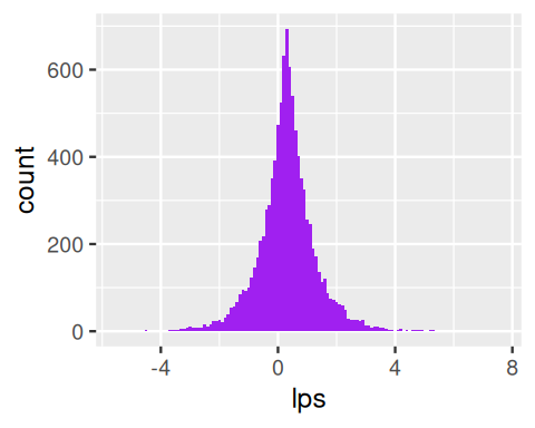
Figure 4.16: Data sampled from a Laplace distribution.

This turns out to be a rather useful distribution. It has well-understood properties and is named after Laplace, who proved that the median is a good estimator of its location parameter $\theta$ and that the median absolute deviation can be used to estimate its scale parameter $\phi$. From the formula in the caption of Figure 4.15 we see that the $L_1$ distance (absolute value of the difference) holds a similar position in the Laplace density as the $L_2$ (square of the difference) does for the normal density.

Conversely, in Bayesian regression⁴, having a Laplace distribution as a prior on the coefficients amounts to an $L_1$ penalty, called the lasso (Tibshirani 1996), while a normal distribution as a prior leads to an $L_2$ penalty, called ridge regression.

⁴ Don’t worry if you are not familiar with this, in that case just skip this sentence.

Question 4.16

Write a random variable whose distribution is the symmetric Laplace as a function of normal and exponential random variables.

Solution

We can write the hierarchical model with variances generated as exponential variables, $W$, as:

\[ X = \sqrt{W} \cdot Z, \qquad W \sim Exp(1), \qquad Z \sim N(0,1). \tag{4.13}\]

Asymmetric Laplace

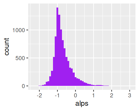
In the Laplace distribution, the variances of the normal components depend on $W$, while the means are unaffected. A useful extension adds another parameter $\theta$ that controls the locations or centers of the components. We generate data alps from a hierarchical model with $W$ an exponential variable; the output shown in Figure 4.17 is a histogram of normal $N(\theta+w\mu,\sigma w)$ random numbers, where the $w$’s themselves were randomly generated from an exponential distribution with mean $1$ as shown in the code:

mu = 0.3; sigma = 0.4; theta = -1
w  = rexp(10000, 1)
alps = rnorm(length(w), theta + mu * w, sigma * sqrt(w))
ggplot(tibble(alps), aes(x = alps)) +
  geom_histogram(fill = "purple", binwidth = 0.1)

Figure 4.17: Histogram of data generated from an asymmetric Laplace distribution – a scale mixture of many normals whose means and variances are dependent. We write $X \sim AL(\theta, \mu, \sigma)$.

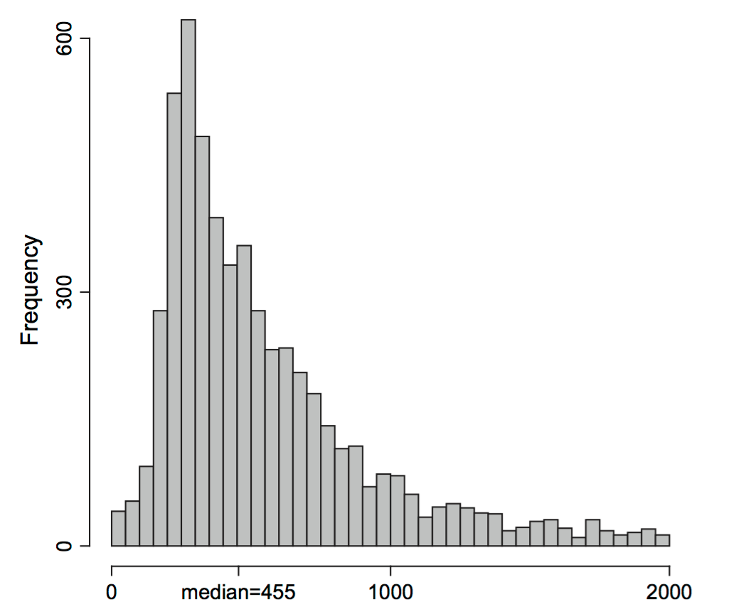
Such hierarchical mixture distributions, where every instance of the data has its own mean and variance, are useful models in many biological settings. Examples are shown in Figure 4.18.

(a) The lengths of the promoters shorter than 2000bp from Saccharomyces cerevisiae as studied by Kristiansson et al. (2009).

Question 4.17

Looking at the log-ratio of gene expression values from a microarray, one gets a distribution as shown on the right of Figure 4.18. How would one explain that the data have a histogram of this form?

The Laplace distribution is an example of where the consideration of the generative process indicates how the variance and mean are linked. The expectation value and variance of an asymmetric Laplace distribution $AL(\theta, \mu, \sigma)$ are

\[ E(X)=\theta+\mu\quad\quad\text{and}\quad\quad\text{var}(X)=\sigma^2+\mu^2. \tag{4.14}\]

Note the variance is dependent on the mean, unless $\mu = 0$ (the case of the symmetric Laplace Distribution). This is the feature of the distribution that makes it useful. Having a mean-variance dependence is very common for physical measurements, be they microarray fluorescence intensities, peak heights from a mass spectrometer, or reads counts from high-throughput sequencing, as we’ll see in the next section.

4.4.2 Infinite mixtures of Poisson variables.

Figure 4.19: How to count the fish in a lake? MC Escher.

A similar two-level hierarchical model is often also needed to model real-world count data. At the lower level, simple Poisson and binomial distributions serve as the building blocks, but their parameters may depend on some underlying (latent) process. In ecology, for instance, we might be interested in variations of fish species in all the lakes in a region. We sample the fish species in each lake to estimate their true abundances, and that could be modeled by a Poisson. But the true abundances will vary from lake to lake. And if we want to see whether, for instance, changes in climate or altitude play a role, we need to disentangle such systematic effects from random lake-to-lake variation. The different Poisson rate parameters $\lambda$ can be modeled as coming from a distribution of rates. Such a hierarchical model also enables us to add supplementary steps in the hierarchy, for instance we could be interested in many different types of fish, model altitude and other environmental factors separately, etc.

Further examples of sampling schemes that are well modeled by mixtures of Poisson variables include applications of high-throughput sequencing, such as RNA-Seq, which we will cover in detail in Chapter 8, or 16S rRNA-Seq data used in microbial ecology.

4.4.3 Gamma distribution: two parameters (shape and scale)

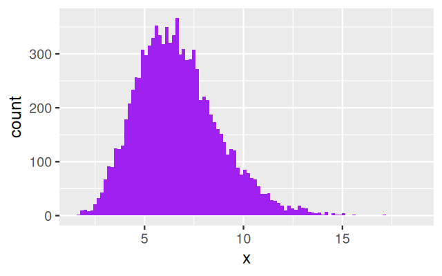
Now we are getting to know a new distribution that we haven’t seen before. The gamma distribution is an extension of the (one-parameter) exponential distribution, but it has two parameters, which makes it more flexible. It is often useful as a building block for the upper level of a hierarchical model. The gamma distribution is positive-valued and continuous. While the density of the exponential has its maximum at zero and then simply decreases towards 0 as the value goes to infinity, the density of the gamma distribution has its maximum at some finite value. Let’s explore it by simulation examples. The histograms in Figure 4.20 were generated by the following lines of code:

ggplot(tibble(x = rgamma(10000, shape = 2, rate = 1/3)),
   aes(x = x)) + geom_histogram(bins = 100, fill= "purple")
ggplot(tibble(x = rgamma(10000, shape = 10, rate = 3/2)),
   aes(x = x)) + geom_histogram(bins = 100, fill= "purple")

Gamma–Poisson mixture: a hierarchical model

Generate a set of parameters: $\lambda_1,\lambda_2,...$ from a gamma distribution.
Use these to generate a set of Poisson($\lambda_i$) random variables, one for each $\lambda_1$.

lambda = rgamma(10000, shape = 10, rate = 3/2)
gp = rpois(length(lambda), lambda = lambda)
ggplot(tibble(x = gp), aes(x = x)) +
  geom_histogram(bins = 100, fill= "purple")

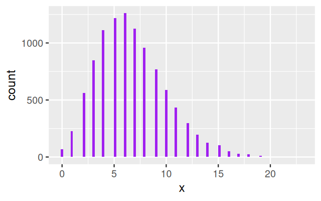
Figure 4.21: Histogram of `gp`, generated via a gamma-Poisson hierachical model.

The resulting values are said to come from a gamma–Poisson mixture. Figure 4.21 shows the histogram of gp.

Question 4.18

Are the values generated from such a gamma–Poisson mixture continuous or discrete ?
What is another name for this distribution? Hint: Try the different distributions provided by the goodfit function from the vcd package.

Solution

library("vcd")
ofit = goodfit(gp, "nbinomial")
plot(ofit, xlab = "")
ofit$par

$size
[1] 10.13849

$prob
[1] 0.6036148

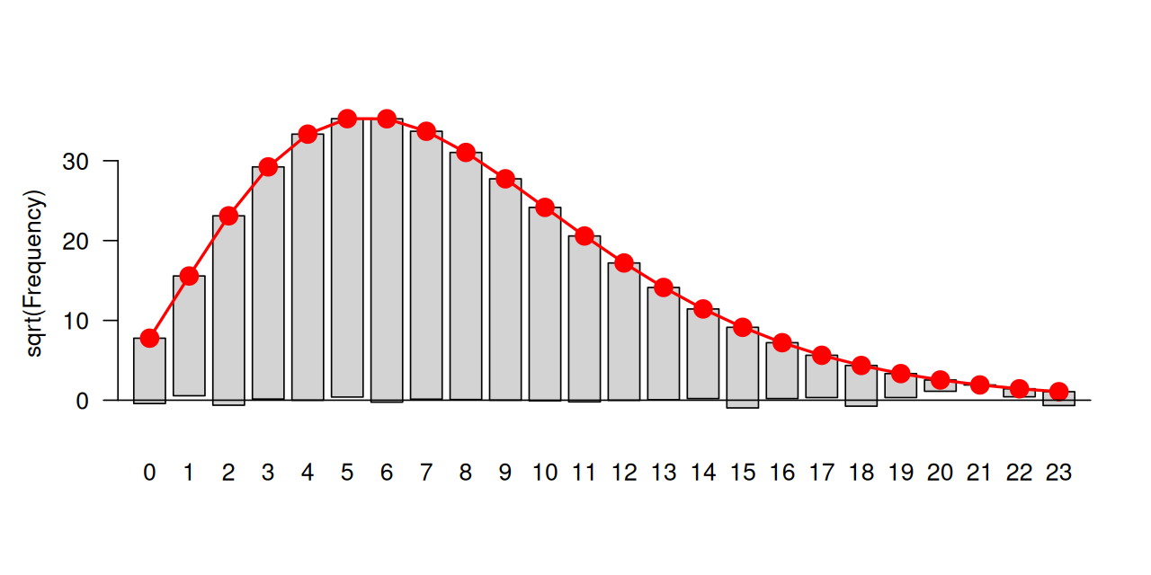
Figure 4.22: Goodness of fit plot. The **rootogram** shows the theoretical probabilities of the gamma-Poisson distribution (a.k.a. negative binomial) as red dots and the square roots of the observed frequencies as the height of the rectangular bars. The bars all end close to the horizontal axis, which indicates a good fit to the negative binomial distribution.

In R, and in some other places, the gamma-Poisson distribution travels under the alias name of negative binomial distribution. The two names are synonyms; the second one alludes to the fact that Equation 4.15 bears some formal similarities to the probabilities of a binomial distribution. The first name, gamma–Poisson distribution, is more indicative of its generating mechanism, and that’s what we will use in the rest of the book. It is a discrete distribution, that means that it takes values only on the natural numbers (in contrast to the gamma distribution, which covers the whole positive real axis). Its probability distribution is

\[ \text{P}(K=k)=\left(\begin{array}{c}k+a-1\\k\end{array}\right) \, p^a \, (1-p)^k, \tag{4.15}\]

which depends on the two parameters $a\in\mathbb{R}^+$ and $p\in[0,1]$. Equivalently, the two parameters can be expressed by the mean $\mu=pa/(1-p)$ and a parameter called the dispersion $\alpha=1/a$. The variance of the distribution depends on these parameters, and is $\mu+\alpha\mu^2$.

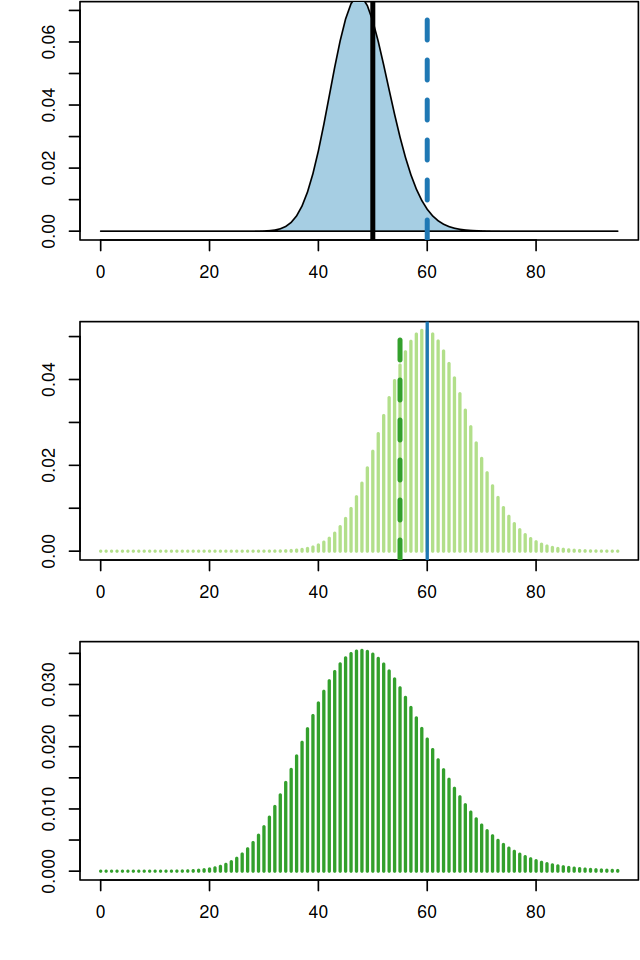
Figure 4.23: Visualization of the hierarchical model that generates the gamma-Poisson distribution. The top panel shows the density of a gamma distribution with mean 50 (vertical black line) and variance 30. Assume that in one particular experimental replicate, the value 60 is realized. This is our latent variable. The observable outcome is distributed according to the Poisson distribution with that rate parameter, shown in the middle panel. In one particular experiment the outcome may be, say, 55, indicated by the dashed green line. Overall, if we repeat these two subsequent random process many times, the outcomes will be distributed as shown in the bottom panel – the gamma-Poisson distribution.

Question 4.19

If you are more interested in analytical derivations than illustrative simulations, try writing out the mathematical derivation of the gamma-Poisson probability distribution.

Solution

Recall that the final distribution is the result of a two step process:

Generate a $\text{gamma}(a,b)$ distributed number, call it $x$, from the density

\[ f_\Gamma(x, a, b)=\frac{b^a}{\Gamma(a)}\,x^{a-1}\,e^{-b x}, \tag{4.16}\]

where $\Gamma$ is the so-called $\Gamma$-function, $\Gamma(a)=\int_0^\infty x^{a-1}\,e^{-x}\,\text{d}x$ (not to be confused with the gamma distribution, even though there is this incidental relation).

Generate a number $k$ from the Poisson distribution with rate $x$. The probability distribution is

\[ f_{\text{Pois}}(k, \lambda=x)=\frac{x^{k}e^{-x}}{k!} \]

If $x$ only took on a finite set of values, we could solve the problem simply by summing over all the possible cases, each weighted by their probability according to $f_\Gamma$. But $x$ is continuous, so we have to write the sum out as an integral instead of a discrete sum. We call the distribution of $K$ the marginal. Its probability mass function is

\[ \begin{aligned} P(K=k)&=&\int_{x=0}^{\infty} \, f_{\text{Pois}}(k, \lambda=x)\; f_\Gamma(x, a, b) \;dx\\ &=& \int_{x=0}^{\infty} \frac{x^{k}e^{-x}}{k!}\;\frac{b^a}{\Gamma(a)} x^{a-1}e^{-bx}\; dx \end{aligned} \]

Collect terms and move terms independent of $x$ outside the integral

\[ P(K=k)=\frac{b^a}{\Gamma(a)\,k!} \int_{x=0}^{\infty} x^{k+a-1}e^{-(b+1)x} dx \]

Because we know the gamma density sums to one: $\int_0^\infty x^{k+a-1}e^{-(b+1)x} dx = \frac{\Gamma(k+a)}{(b+1)^{k+a}}$

\[ \begin{aligned} P(K=k) &=&\frac{\Gamma(k+a)}{\Gamma(a)\Gamma(k+1)}\frac{b^a}{(b+1)^{a}(b+1)^k} ={k+a-1\choose k}\left(\frac{b}{b+1}\right)^a\left(1-\frac{b}{b+1}\right)^k \end{aligned} \]

where in the last line we used that $\Gamma(v+1)=v!$. This is the same as Equation (4.15), the gamma-Poisson with size parameter $a$ and probability $p=\frac{b}{b+1}$.

4.4.4 Variance stabilizing transformations

A key issue we need to control when we analyse experimental data is how much variability there is between repeated measurements of the same underlying true value, i.e., between replicates. This will determine whether and how well we can see any true differences, i.e., between different conditions. Data that arise through the type of hierarchical models we have studied in this chapter often turn out to have very heterogeneous variances, and this can be a challenge. We will see how in such cases variance-stabilizing transformations (Anscombe 1948) can help. Let’s start with a series of Poisson variables with rates from 10 to 100:

Note how we construct the dataframe (or, more precisely, the tibble) simdat: the output of the lapply loop is a list of tibbles, one for each value of lam. With the pipe operator |> we send it to the function bind_rows (from the dplyr package). The result is a dataframe of all the list elements neatly stacked on top of each other.

simdat = lapply(seq(10, 100, by = 10), function(lam)
    tibble(n = rpois(200, lambda = lam),
           `sqrt(n)` = sqrt(n),
       lambda = lam)) |>
  bind_rows() |>
  tidyr::pivot_longer(cols = !lambda)
ggplot(simdat, aes(x = factor(lambda), y = value)) + xlab(expression(lambda)) +
  geom_violin() + facet_grid(rows = vars(name), scales = "free")

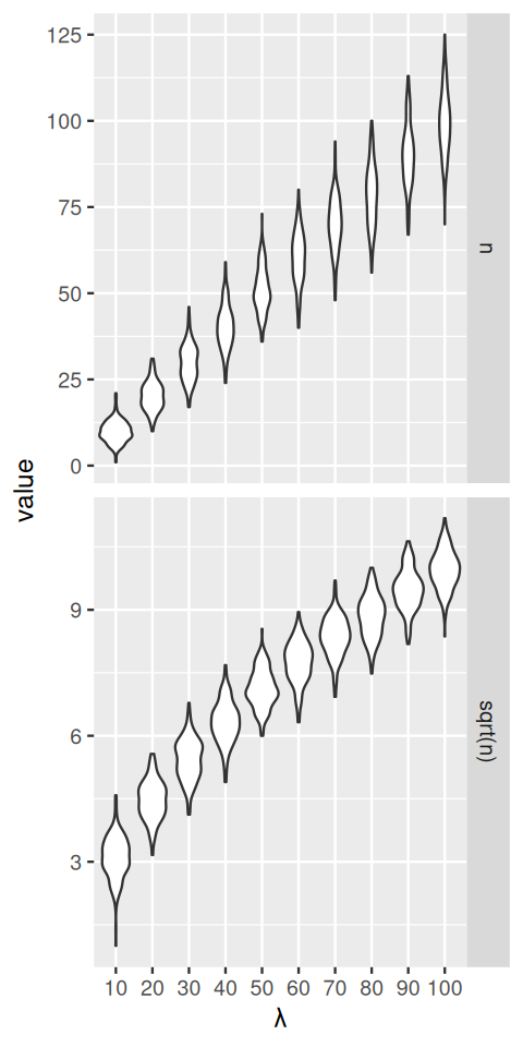
Figure 4.24: Poisson distributed measurement data, for eight different choices of the mean `lambda`. In the upper panel, the $y$-axis is proportional to the data; in the lower panel, it is on a square-root scale. Note how the distribution widths change in the first case, but less so in the second.

The data that we see in the upper panel of Figure 4.24 are an example of what is called heteroscedasticity: the standard deviations (or, equivalently, the variance) of our data is different in different regions of our data space. In particular, it increases along the $x$-axis, with the mean. For the Poisson distribution, we indeed know that the standard deviation is the square root of the mean; for other types of data, there may be other dependencies. This can be a problem if we want to apply subsequent analysis techniques (for instance, regression, or a statistical test) that are based on assuming that the variances are the same. In Figure 4.24, the numbers of replicates for each value of lambda are quite large. In practice, this is not always the case. Moreover, the data are usually not explicitly stratified by a known mean as in our simulation, so the heteroskedasticity may be harder to see, even though it is there. However, as we see in the lower panel of Figure 4.24, if we simply apply the square root transformation, then the transformed variables will have approximately the same variance. This works even if we do not know the underlying mean for each observation, the square root transformation does not need this information. We can verify this more quantitatively, as in the following code, which shows the standard deviations of the sampled values n and sqrt(n) for the difference choices of lambda.

The standard deviation of the square root transformed values is consistently around 0.5, so we would use the transformation 2*sqrt(n) to achieve unit variance.

summarise(group_by(simdat, name, lambda), sd(value)) |> tidyr::pivot_wider(values_from = `sd(value)`)

# A tibble: 10 × 3
   lambda     n `sqrt(n)`
    <dbl> <dbl>     <dbl>
 1     10  3.02     0.490
 2     20  4.40     0.501
 3     30  5.57     0.521
 4     40  6.90     0.543
 5     50  7.36     0.522
 6     60  8.30     0.538
 7     70  9.00     0.546
 8     80  8.94     0.504
 9     90  8.89     0.475
10    100 10.2      0.505

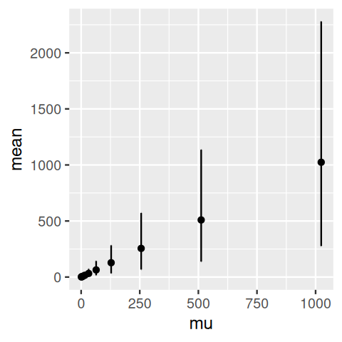
Another example, now using the gamma-Poisson distribution, is shown in Figure 4.25. We generate gamma-Poisson variables u⁵ and plot the 95% confidence intervals around the mean.

⁵ To catch a greater range of values for the mean value mu, without creating too dense a sequence, we use a geometric series: $\mu_{i+1} = 2\mu_i$.

muvalues = 2^seq(0, 10, by = 1)
simgp = lapply(muvalues, function(mu) {
  u = rnbinom(n = 1e4, mu = mu, size = 4)
  tibble(mean = mean(u), sd = sd(u),
         lower = quantile(u, 0.025),
         upper = quantile(u, 0.975),
         mu = mu)
  } ) |> bind_rows()
head(as.data.frame(simgp), 2)

    mean       sd lower upper mu
1 0.9844 1.104843     0     4  1
2 1.9726 1.725847     0     6  2

ggplot(simgp, aes(x = mu, y = mean, ymin = lower, ymax = upper)) +
  geom_point() + geom_errorbar()

Figure 4.25: gamma-Poisson distributed measurement data, for a range of $\mu$ from 1 to 1024.

Question 4.20

How can we find a transformation for these data that stabilizes the variance, similar to the square root function for the Poisson distributed data?

Solution

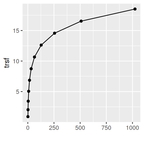
If we divide the values that correspond to mu[1] (and which are centered around simgp$mean[1]) by their standard deviation simgp$sd[1], the values that correspond to mu[2] (and which are centered around simgp$mean[2]) by their standard deviation simgp$sd[2], and so on, then the resulting values will have, by construction, a standard deviation (and thus variance) of 1. And rather than defining 11 separate transformations, we can achieve our goal by defining one single piecewise linear and continuous function that has the appropriate slopes at the appropriate values.

simgp = mutate(simgp,
  slopes = 1 / sd,
  trsf   = cumsum(slopes * mean))
ggplot(simgp, aes(x = mean, y = trsf)) +
  geom_point() + geom_line() + xlab("")

Figure 4.26: Piecewise linear function that stabilizes the variance of the data in Figure 4.25.

We see in Figure 4.26 that this function has some resemblance to a square root function in particular at its lower end. At the upper end, it seems to look more like a logarithm. The more mathematically inclined will see that an elegant extension of these numerical calculations can be done through a little calculus known as the delta method, as follows.

Call our transformation function $g$, and assume it’s differentiable (that’s not a very strong assumption: pretty much any function that we might consider reasonable here is differentiable). Also call our random variables $X_i$, with means $\mu_i$ and variances $v_i$, and we assume that $v_i$ and $\mu_i$ are related by a functional relationship $v_i = v(\mu_i)$. Then, for values of $X_i$ in the neighborhood of its mean $\mu_i$,

\[ g(X_i) = g(\mu_i) + g'(\mu_i) (X_i-\mu_i) + ... \tag{4.17}\]

where the dots stand for higher order terms that we can neglect. The variances of the transformed values are then

\[ \begin{align} \text{Var}(g(X_i)) &\simeq g'(\mu_i)^2\\ \text{Var}(X_i) &= g'(\mu_i)^2 \, v(\mu_i), \end{align} \tag{4.18}\]

where we have used the rules $\text{Var}(X-c)=\text{Var}(X)$ and $\text{Var}(cX)=c^2\,\text{Var}(X)$ that hold whenever $c$ is a constant number. Requiring that this be constant leads to the differential equation

\[ g'(x) = \frac{1}{\sqrt{v(x)}}. \tag{4.19}\]

For a given mean-variance relationship $v(\mu)$, we can solve this for the function $g$. Let’s check this for some simple cases:

if $v(\mu)=\mu$ (Poisson), we recover $g(x)=\sqrt{x}$, the square root transformation.
If $v(\mu)=\alpha\,\mu^2$, solving the differential equation 4.19 gives $g(x)=\log(x)$. This explains why the logarithm transformation is so popular in many data analysis applications: it acts as a variance stabilizing transformation whenever the data have a constant coefficient of variation, that is, when the standard deviation is proportional to the mean.

Question 4.21

What is the variance-stabilizing transformation associated with $v(\mu) = \mu + \alpha\,\mu^2$?

Solution

To solve the differential equation 4.19 with this function $v(\cdot)$, we need to compute the integral

\[\label{eq:} \int \frac{dx}{\sqrt{x + \alpha x^2}}. \tag{4.20}\]

A closed form expression can be looked up in a reference table such as (Bronštein and Semendjajew 1979). These authors provide the general solution

\[ \int \frac{dx}{\sqrt{ax^2+bx+c}} = \frac{1}{\sqrt{a}} \ln\left(2\sqrt{a(ax^2+bx+c)}+2ax+b\right) + \text{const.}, \tag{4.21}\]

into which we can plug in our special case $a=\alpha$, $b=1$, $c=0$, to obtain the variance-stabilizing transformation

\[ \begin{align} g_\alpha(x) &= \frac{1}{2\sqrt{\alpha}} \ln\left(2\sqrt{\alpha x (\alpha x+1)} + 2\alpha x + 1\right) \\ &= \frac{1}{2\sqrt{\alpha}} {\displaystyle \operatorname {arcosh}} (2\alpha x+1).\\ \end{align} \tag{4.22}\]

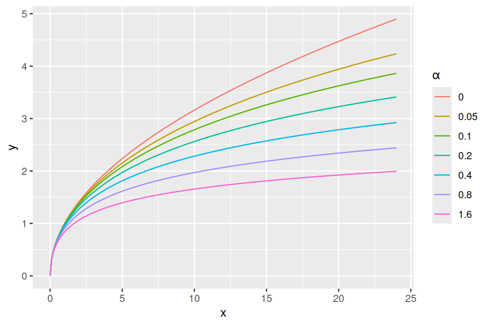
For the second line in Equation 4.22, we used the identity ${\displaystyle \operatorname {arcosh}}(z) = \ln\left(z+\sqrt{z^2-1}\right)$. In the limit of $\alpha\to0$, we can use the linear approximation $\ln(1+\varepsilon)=\varepsilon+O(\varepsilon^2)$ to see that $g_0(x)=\sqrt{x}$. Note that if $g_\alpha$ is a variance-stabilizing transformation, then so is $ug_\alpha+v$ for any pair of numbers $u$ and $v$, and we have used this freedom to insert an extra factor $\frac{1}{2}$ for reasons that become apparent in the following. You can verify that the function $g_\alpha$ from Equation 4.22 fulfills condition 4.19 by computing its derivative, which is an elementary calculation. We can plot it:

f = function(x, a) 
  ifelse (a==0, 
    sqrt(x), 
    log(2*sqrt(a) * sqrt(x*(a*x+1)) + 2*a*x+1) / (2*sqrt(a)))
x  = seq(0, 24, by = 0.1)
df = lapply(c(0, 0.05*2^(0:5)), function(a) 
  tibble(x = x, a = a, y = f(x, a))) %>% bind_rows()
ggplot(df, aes(x = x, y = y, col = factor(a))) + 
  geom_line() + labs(col = expression(alpha))

Figure 4.27: Graph of the function Equation 4.22 for different choices of $\alpha$.

and empirically verify the equivalence of two terms in Equation 4.22:

f2 = function(x, a) ifelse (a==0, sqrt(x), acosh(2*a*x + 1) / (2*sqrt(a)))  
with(df, max(abs(f2(x,a) - y)))

[1] 8.881784e-16

As we see in Figure 4.27, for small values of $x$, $g_\alpha(x)\approx \sqrt{x}$ (independently of $\alpha$), whereas for large values ($x\to\infty$) and $\alpha>0$, it behaves like a logarithm:

\[ \begin{align} &\frac{1}{2\sqrt{\alpha}}\ln\left(2\sqrt{\alpha\left(\alpha x^2+x\right)}+2\alpha x+1\right)\\ \approx&\frac{1}{2\sqrt{\alpha}} \ln\left(2\sqrt{\alpha^2x^2}+2\alpha x\right)\\ =&\frac{1}{2\sqrt{\alpha}}\ln\left(4\alpha x\right)\\ =&\frac{1}{2\sqrt{\alpha}}\ln x+\text{const.} \end{align} \]

We can verify this empirically by, say,

  a = c(0.2, 0.5, 1)
  f(1e6, a)

[1] 15.196731 10.259171  7.600903

  1/(2*sqrt(a)) * (log(1e6) + log(4*a))

[1] 15.196728 10.259170  7.600902

4.5 Summary of this chapter

We have given motivating examples and ways of using mixtures to model biological data. We saw how the EM algorithm is an interesting example of fitting a difficult-to-estimate probabilistic model to data by iterating between partial, simpler problems.

Finite mixture models

We have seen how to model mixtures of two or more normal distributions with different means and variances. We have seen how to decompose a given sample of data from such a mixture, even without knowing the latent variable, using the EM algorithm. The EM approach requires that we know the parametric form of the distributions and the number of components. In Chapter 5, we will see how we can find groupings in data even without relying on such information – this is then called clustering. We can keep in mind that there is a strong conceptual relationship between clustering and mixture modeling.

Common infinite mixture models

Infinite mixture models are good for constructing new distributions (such as the gamma-Poisson or the Laplace) out of more basic ones (such as binomial, normal, Poisson). Common examples are

mixtures of normals (often with a hierarchical model on the means and the variances);
beta-binomial mixtures – where the probability $p$ in the binomial is generated according to a $\text{beta}(a, b)$ distribution;
gamma-Poisson for read counts (see Chapter 8);
gamma-exponential for PCR.

Applications

Mixture models are useful whenever there are several layers of experimental variability. For instance, at the lowest layer, our measurement precision may be limited by basic physical detection limits, and these may be modeled by a Poisson distribution in the case of a counting-based assay, or a normal distribution in the case of the continuous measurement. On top of there may be one (or more) layers of instrument-to-instrument variation, variation in the reagents, operator variaton etc.

Mixture models reflect that there is often heterogeneous amounts of variability (variances) in the data. In such cases, suitable data transformations, i.e., variance stabilizing transformations, are necessary before subsequent visualization or analysis. We’ll study in depth an example for RNA-Seq in Chapter 8, and this also proves useful in the normalization of next generation reads in microbial ecology (McMurdie and Holmes 2014).

Another important application of mixture modeling is the two-component model in multiple testing – we will come back to this in Chapter 6.

The ECDF and bootstrapping

We saw that by using the observed sample as a mixture we could generate many simulated samples that inform us about the sampling distribution of an estimate. This method is called the bootstrap and we will return to it several times, as it provides a way of evaluating estimates even when a closed form expression is not available (we say it is non-parametric).

4.6 Further reading

A useful book-long treatment of finite mixture models is by McLachlan and Peel (2004); for the EM algorithm, see also the book by McLachlan and Krishnan (2007). A recent book that presents all EM type algorithms within the Majorize-Minimization (MM) framework is by Lange (2016).

There are in fact mathematical reasons why many natural phenomena can be seen as mixtures: this occurs when the observed events are exchangeable (the order in which they occur doesn’t matter). The theory underlying this is quite mathematical, a good way to start is to look at the Wikipedia entry and the paper by Diaconis and Freedman (1980).

In particular, we use mixtures for high-throughput data. You will see examples in Chapters 8 and 11.

The bootstrap can be used in many situations and is a very useful tool to know about, a friendly treatment is given in (B. Efron and Tibshirani 1993).

A historically interesting paper is the original article on variance stabilization by Anscombe (1948), who proposed ways of making variance stabilizing transformations for Poisson and gamma-Poisson random variables. Variance stabilization is explained using the delta method in many standard texts in theoretical statistics, e.g., those by Rice (2006, chap. 6) and Kéry and Royle (2015, 35).

Kéry and Royle (2015) provide a nice exploration of using R to build hierarchical models for abundance estimation in niche and spatial ecology.

4.7 Exercises

Exercise 4.1

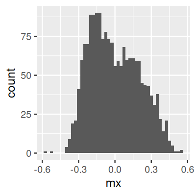
The EM algorithm step by step. As an example dataset, we use the values in the file Myst.rds. As always, it is a good idea to first visualize the data. The histogram is shown in Figure 4.28. We are going to model these data as a mixture of two normal distributions with unknown means and standard deviations, and unknown mixture fraction. We’ll call the two components A and B.

mx = readRDS("../data/Myst.rds")$yvar
str(mx)

 num [1:1800] 0.3038 0.0596 -0.0204 0.1849 0.2842 ...

ggplot(tibble(mx), aes(x = mx)) + geom_histogram(binwidth = 0.025)

We start by randomly assigning the membership weights for each of the values in mx for each of the components

wA = runif(length(mx))
wB = 1 - wA

We also need to set up some housekeeping variables: iter counts over the iterations of the EM algorithm; loglik stores the current log-likelihood; delta stores the change in the log-likelihood from the previous iteration to the current one. We also define the parameters tolerance, miniter and maxiter of the algorithm.

iter      = 0
loglik    = -Inf
delta     = +Inf
tolerance = 1e-12
miniter   = 50
maxiter   = 1000

Study the code below and answer the following questions:

Which lines correspond to the E-step, which to the M-step?
What is the role of tolerance, miniter and maxiter?
Compare the result of what we are doing here to the output of the normalmixEM function from the mixtools package.

while((delta > tolerance) && (iter <= maxiter) || (iter < miniter)) {
  lambda = mean(wA)
  muA = weighted.mean(mx, wA)
  muB = weighted.mean(mx, wB)
  sdA = sqrt(weighted.mean((mx - muA)^2, wA))
  sdB = sqrt(weighted.mean((mx - muB)^2, wB))

  pA   =    lambda    * dnorm(mx, mean = muA, sd = sdA)
  pB   = (1 - lambda) * dnorm(mx, mean = muB, sd = sdB)
  ptot = pA + pB
  wA   = pA / ptot
  wB   = pB / ptot

  loglikOld = loglik
  loglik = sum(log(pA + pB))
  delta = abs(loglikOld - loglik)
  iter = iter + 1
}
iter

[1] 437

c(lambda, muA, muB, sdA, sdB)

[1]  0.4756 -0.1694  0.1473  0.0983  0.1498

Figure 4.28: Histogram of `mx`, our example data for the EM algorithm.

Solution

The first five lines in the while loop implement the Maximization step. Given the current values of wA and wB, we estimate the parameters of the mixture model using the maximum-likelihood estimators: the mixture fraction lambda by the mean of wA, and the parameters of the two normal distribution components (muA, sdA) and (muB, sdB) by the sample means and the sample standard deviations. To take into account the membership weights, we use the weighted mean (function weighted.mean) and standard deviation.

Next comes the Expectation step. For each of the elements in the data vector mx, we compute the probability densities pA and pB for the generative distribution models A and B, using the normal density function dnorm, weighted by the mixture fractions lambda and (1-lambda), respectively. From this, we compute the updated membership weights wA and wB, according to Equation 4.5.

Given the membership weights and the parameters, the logarithmic likelihood loglik is easily computed, and the while loop iterates these steps.

The termination criterion for the loop is based on delta, the change in the likelihood. The loop can end if this becomes smaller than tolerance. This is a simple way of checking whether the algorithm has converged. The additional conditions on iter make sure that at least miniter iterations are run, and that the loop always stops after maxiter iterations. The latter is to make sure that the loop terminates in finite time no matter what. (“Professional” implementations of such iterative algorithms typically work a bit harder to decide what is the best time to stop.)

Finally, let’s compare our estimates to those from the function normalmixEM from the mixtools package.

gm = mixtools::normalmixEM(mx, k = 2)

number of iterations= 230

with(gm, c(lambda[1], mu, sigma))

[1]  0.4757 -0.1694  0.1473  0.0983  0.1498

Exercise 4.2

Why do we often consider the logarithm of the likelihood rather than the likelihood? E.g., in the EM code above, why did we work with the probabilities on the logarithmic scale?

Solution

Likelihoods often (whenever the data points are sampled independently) take the form of a product. This is, for instance, the case in Equation 4.4. Calculating the derivative, for likelihood optimisation, would then require application of the product rule. On the logarithmic scale, the product turns into a sum, and the derivative of a sum is simply the sum of the derivatives of the individual summands.

An additional reason comes from the way computers implement arithmetic. They commonly use a floating point representation of numbers with a finite number of bits. E.g., the IEEE 754-2008 standard uses 64 bits for a double-precision number: 1 bit for the sign, 52 for the mantissa (also called significand), 11 for the exponent. Multiplication between such numbers implies addition of the exponents, but the range of the exponent is only $0$ to $2^{11}-1=2047$. Even likelihoods that involve only a few hundred data points can lead to arithmetic overflow or other problems with precision. On the logarithmic scale, where the product is a sum, the workload tends to be better distributed between mantissa and exponent, and log-likelihoods even with millions of data points to be handled with reasonable precision.

See also Gregory Gundersen’s post on the Log-Sum-Exp Trick for normalizing vectors of log probabilities.

Exercise 4.3

Compare the theoretical values of the gamma-Poisson distribution with parameters given by the estimates in ofit$par in Section 4.4.3 to the data used for the estimation using a QQ-plot.

Exercise 4.4

Mixture modeling examples for regression. The flexmix package (Grün, Scharl, and Leisch 2012) enables us to cluster and fit regressions to the data at the same time. The standard M-step FLXMRglm of flexmix is an interface to R’s generalized linear modeling facilities (the glm function). Load the package and an example dataset.

library("flexmix")
data("NPreg")

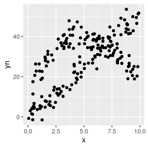
First, plot the data and try to guess how the points were generated.
Fit a two component mixture model using the commands

m1 = flexmix(yn ~ x + I(x^2), data = NPreg, k = 2)

Look at the estimated parameters of the mixture components and make a truth table that cross-classifies true classes versus cluster memberships. What does the summary of the object m1 show us?
Plot the data again, this time coloring each point according to its estimated class.

Solution

ggplot(NPreg, aes(x = x, y = yn)) + geom_point()

Figure 4.29: The points seem to come from two different generative processes, one is linear; the other quadratic.

The components are:

modeltools::parameters(m1, component = 1)

                     Comp.1
coef.(Intercept) 14.7165473
coef.x            9.8466895
coef.I(x^2)      -0.9683509
sigma             3.4800086

modeltools::parameters(m1, component = 2)

                      Comp.2
coef.(Intercept) -0.20993466
coef.x            4.81768211
coef.I(x^2)       0.03617263
sigma             3.47611967

The parameter estimates of both components are close to the true values. A cross-tabulation of true classes and cluster memberships can be obtained by

table(NPreg$class, modeltools::clusters(m1))

For our example data, the ratios of both components are approximately 0.7, indicating the overlap of the classes at the cross-section of line and parabola.

summary(m1)

The summary shows the estimated prior probabilities $\hat\pi_k$, the number of observations assigned to the two clusters, the number of observations where $p_{nk}>\delta$ (with a default of $\delta=10^{-4}$), and the ratio of the latter two numbers. For well-separated components, a large proportion of observations with non-vanishing posteriors $p_{nk}$ should be assigned to their cluster, giving a ratio close to 1.

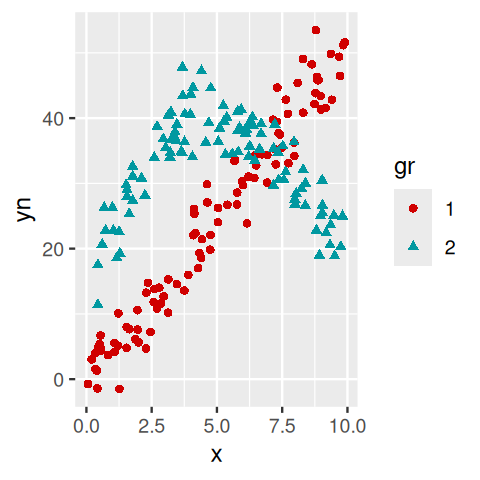
NPreg = mutate(NPreg, gr = factor(class))
ggplot(NPreg, aes(x = x, y = yn, group = gr)) +
   geom_point(aes(colour = gr, shape = gr)) +
   scale_colour_hue(l = 40, c = 180)

Figure 4.30: Regression example using `flexmix` with the points colored according to their estimated class. You can see that at the intersection we have an `identifiability’ problem: we cannot distinguish points that belong to the straight line from ones that belong to the parabole.

Exercise 4.5

Other hierarchical noise models:
Find two papers that explore the use of other infinite mixtures for modeling molecular biology technological variation.

Solution

The paper by Chen, Xie, and Story (2011) explores an exponential-Poisson model for modeling background noise in bead arrays. Wills et al. (2013) compares several Poisson mixture models.

Anscombe, Francis J. 1948. “The Transformation of Poisson, Binomial and Negative-Binomial Data.” Biometrika, 246–54.

Bishop, Christopher M. 2006. Pattern Recognition and Machine Learning. Springer.

Bronštein, Il’ja N., and Konstantin A Semendjajew. 1979. Taschenbuch Der Mathematik. B.G. Teubner Verlagsgesellschaft, Leipzig; Verlag Nauka, Moscow.

Bulmer, Michael George. 2003. Francis Galton: Pioneer of Heredity and Biometry. JHU Press.

Chen, Min, Yang Xie, and Michael Story. 2011. “An Exponential-Gamma Convolution Model for Background Correction of Illumina BeadArray Data.” Communications in Statistics-Theory and Methods 40 (17): 3055–69.

Diaconis, Persi, and David Freedman. 1980. “Finite Exchangeable Sequences.” The Annals of Probability, 745–64.

Diaconis, Persi, and Susan Holmes. 1994. “Gray Codes for Randomization Procedures.” Statistics and Computing 4 (4): 287–302.

Efron, Bradley, and Robert J Tibshirani. 1994. An Introduction to the Bootstrap. CRC press.

Efron, B., and R. Tibshirani. 1993. An Introduction to the Bootstrap. Chapman & Hall/CRC.

Grün, Bettina, Theresa Scharl, and Friedrich Leisch. 2012. “Modelling Time Course Gene Expression Data with Finite Mixtures of Linear Additive Models.” Bioinformatics 28 (2): 222–28. https://doi.org/10.1093/bioinformatics/btr653.

Hoeting, Jennifer A, David Madigan, Adrian E Raftery, and Chris T Volinsky. 1999. “Bayesian Model Averaging: A Tutorial.” Statistical Science, 382–401.

Kéry, Marc, and J Andrew Royle. 2015. Applied Hierarchical Modeling in Ecology: Analysis of Distribution, Abundance and Species Richness in r and BUGS: Volume 1: Prelude and Static Models. Academic Press.

Kristiansson, Erik, Michael Thorsen, Markus J Tamás, and Olle Nerman. 2009. “Evolutionary Forces Act on Promoter Length: Identification of Enriched Cis-Regulatory Elements.” Molecular Biology and Evolution 26 (6): 1299–1307.

Kuan, Pei Fen, Dongjun Chung, Guangjin Pan, James A Thomson, Ron Stewart, and Sündüz Keleş. 2011. “A Statistical Framework for the Analysis of ChIP-Seq Data.” Journal of the American Statistical Association 106 (495): 891–903.

Lange, Kenneth. 2016. MM Optimization Algorithms. SIAM.

McLachlan, Geoffrey, and Thriyambakam Krishnan. 2007. The EM Algorithm and Extensions. Vol. 382. John Wiley & Sons.

McLachlan, Geoffrey, and David Peel. 2004. Finite Mixture Models. John Wiley & Sons.

McMurdie, Paul J, and Susan Holmes. 2014. “Waste Not, Want Not: Why Rarefying Microbiome Data Is Inadmissible.” PLoS Computational Biology 10 (4): e1003531.

Purdom, Elizabeth, and Susan P Holmes. 2005. “Error Distribution for Gene Expression Data.” Statistical Applications in Genetics and Molecular Biology 4 (1).

Rice, John. 2006. Mathematical Statistics and Data Analysis. Cengage Learning.

Shalizi, Cosma. 2017. Advanced Data Analysis from an Elementary Point of View. Cambridge University Press. https://www.stat.cmu.edu/~cshalizi/ADAfaEPoV/ADAfaEPoV.pdf.

Slonim, Noam, Gurinder Singh Atwal, Gašper Tkačik, and William Bialek. 2005. “Information-Based Clustering.” PNAS 102 (51): 18297–302.

Tibshirani, Robert. 1996. “Regression Shrinkage and Selection via the Lasso.” Journal of the Royal Statistical Society. Series B (Methodological), 267–88.

Wills, Quin F, Kenneth J Livak, Alex J Tipping, Tariq Enver, Andrew J Goldson, Darren W Sexton, and Chris Holmes. 2013. “Single-Cell Gene Expression Analysis Reveals Genetic Associations Masked in Whole-Tissue Experiments.” Nature Biotechnology 31 (8): 748–52.

Zeileis, Achim, Christian Kleiber, and Simon Jackman. 2008. “Regression Models for Count Data in R.” Journal of Statistical Software 27 (8). http://www.jstatsoft.org/v27/i08/.

Page built at 08:54 on 2024-11-22 using R version 4.4.1 (2024-06-14)

Support for maintaining the online version of this book is provided by de.NBI

For website support please contact msmith@embl.de