turtles = read.table("../data/PaintedTurtles.txt", header = TRUE)
turtles[1:4, ]
sex length width height
1 f 98 81 38
2 f 103 84 38
3 f 103 86 42
4 f 105 86 40
Many datasets consist of several variables measured on the same set of subjects: patients, samples, or organisms. For instance, we may have biometric characteristics such as height, weight, age as well as clinical variables such as blood pressure, blood sugar, heart rate, and genetic data for, say, a thousand patients. The raison d’être for multivariate analysis is the investigation of connections or associations between the different variables measured. Usually the data are reported in a tabular data structure with one row for each subject and one column for each variable. In the following, we will focus on the special case where each of the variables is numeric, so we can represent the data structure as a matrix in R.
If the columns of the matrix are all independent of each other (unrelated), we can simply study each column separately and do standard “univariate” statistics on them one by one; there would be no benefit in studying them as a matrix.
More often, there will be patterns and dependencies. For instance, in the biology of cells, we know that the proliferation rate will influence the expression of many genes simultaneously. Studying the expression of 25,000 gene (columns) on many samples (rows) of patient-derived cells, we notice that many of the genes act together, either that they are positively correlated or that they are anti-correlated. We would miss a lot of important information if we were to only study each gene separately. Important connections between genes are detectable only if we consider the data as a whole: each row representing the many measurements made on the same observational unit. However, having 25,000 dimensions of variation to consider at once is daunting; we will show how to reduce our data to a smaller number of most important dimensions1 without losing too much information.
1 We will elaborate this idea of dimension reduction in much more detail below. For the time being, remember we live in a four-dimensional world.
This chapter presents many examples of multivariate data matrices that we encounter in high-throughput experiments, as well as some more elementary examples that we hope will enhance your intuition. We will focus in this chapter on Principal Component Analysis, abbreviated as PCA, a dimension reduction method. We will provide geometric explanations of the algorithm as well as visualizations that help interpret the output of PCA analyses.
In this chapter we will:
See examples of matrices that come up in the study of biological data.
Perform dimension reduction to understand correlations between variables.
Preprocess, rescale and center the data before starting a multivariate analysis.
Build new variables, called principal components (PC), that are more useful than the original measurements.
See what is “under the hood” of PCA: the singular value decomposition of a matrix.
Visualize what this decomposition achieves and learn how to choose the number of principal components.
Run through a complete PCA analysis from start to finish.
Project factor covariates onto the PCA map to enable a more useful interpretation of the results.
First, let’s look at a set of examples of rectangular matrices used to represent tables of measurements. In each matrix, the rows and columns represent specific entities.
Turtles: A simple data set that will help us understand the basic principles is a matrix of three dimensions of biometric measurements on painted turtles (Jolicoeur and Mosimann 1960).
turtles = read.table("../data/PaintedTurtles.txt", header = TRUE)
turtles[1:4, ] sex length width height
1 f 98 81 38
2 f 103 84 38
3 f 103 86 42
4 f 105 86 40The last three columns are length measurements (in millimetres), whereas the first column is a factor variable that tells us the sex of each animal.
Athletes: This matrix is an interesting example from the sports world. It reports the performances for 33 athletes in the ten disciplines of the decathlon: m100, m400 and m1500 are times in seconds for the 100 meters, 400 meters, and 1500 meters respectively; m110 is the time to finish the 110 meters hurdles; pole is the pole-vault height, and high and long are the results of the high and long jumps, all in meters; weight, disc, and javel are the lengths in meters the athletes were able to throw the weight, discus and javelin. Here are these variables for the first three athletes:
data("olympic", package = "ade4")
athletes_1 = setNames(
  olympic$tab,
  c(
    "m100",
    "long",
    "weight",
    "high",
    "m400",
    "m110",
    "disc",
    "pole",
    "javel",
    "m1500"
  )
)
athletes_1[1:3, ]
m100 long weight high m400 m110 disc pole javel m1500
1 11.2 7.43 15.5 2.27 48.9 15.1 49.3 4.7 61.3 269
2 10.9 7.45 15.0 1.97 47.7 14.5 44.4 5.1 61.8 273
3 11.2 7.44 14.2 1.97 48.3 14.8 43.7 5.2 64.2 263Cell Types: Holmes et al. (2005) studied gene expression profiles of sorted T-cell populations from different subjects. The columns are a subset of gene expression measurements, they correspond to 156 genes that show differential expression between cell types.
load("../data/Msig3transp.RData")
round(Msig3transp, 2)[1:5, 1:6]
X3968 X14831 X13492 X5108 X16348 X585
HEA26_EFFE_1 -2.61 -1.19 -0.06 -0.15 0.52 -0.02
HEA26_MEM_1 -2.26 -0.47 0.28 0.54 -0.37 0.11
HEA26_NAI_1 -0.27 0.82 0.81 0.72 -0.90 0.75
MEL36_EFFE_1 -2.24 -1.08 -0.24 -0.18 0.64 0.01
MEL36_MEM_1 -2.68 -0.15 0.25 0.95 -0.20 0.17Bacterial Species Abundances: Matrices of counts are used in microbial ecology studies (as we saw in Chapter 4). Here the columns represent different species (or operational taxonomic units, OTUs) of bacteria, which are identified by numerical tags. The rows are labeled according to the samples in which they were measured, and the (integer) numbers represent the number of times of each of the OTUs was observed in each of the samples.
data("GlobalPatterns", package = "phyloseq")
GPOTUs = as.matrix(t(phyloseq::otu_table(GlobalPatterns)))
GPOTUs[1:4, 6:13]
OTU Table: [4 taxa and 8 samples]
taxa are rows
246140 143239 244960 255340 144887 141782 215972 31759
CL3 0 7 0 153 3 9 0 0
CC1 0 1 0 194 5 35 3 1
SV1 0 0 0 0 0 0 0 0
M31Fcsw 0 0 0 0 0 0 0 0
mRNA reads: RNA-Seq transcriptome data report the number of sequence reads matching each gene2 in each of several biological samples. We will study this type of data in detail in Chapter 8
2 Or sub-gene structures, such as exons.
library("SummarizedExperiment")
data("airway", package = "airway")
assay(airway)[1:3, 1:4]
SRR1039508 SRR1039509 SRR1039512 SRR1039513
ENSG00000000003 679 448 873 408
ENSG00000000005 0 0 0 0
ENSG00000000419 467 515 621 365It is customary in the RNA-Seq field—and so it is for the airway data above—to report the genes in the rows and the samples in the columns. Compared to the other matrices we look at here, this is transposed: rows and columns are swapped. Such different conventions easily lead to errors, so they are worthwhile paying attention to3. Proteomic profiles: Here, the columns are aligned mass spectroscopy peaks or molecules identified through their \(m/z\)-ratios; the entries in the matrix are the measured intensities4.
3 The Bioconductor project tries to help users and developers to avoid such ambiguities by defining data containers in which such conventions are explicitly fixed. In Chapter 8, we will see the example of the SummarizedExperiment class.
4 More details can be found, e.g., on Wikipedia.
metab = t(as.matrix(read.csv("../data/metabolites.csv", row.names = 1)))
metab[1:4, 1:4]
146.0985388 148.7053275 310.1505057 132.4512963
KOGCHUM1 29932 17056 1133 786
KOGCHUM2 94068 74632 28241 5232
KOGCHUM3 146411 147789 64950 10283
WTGCHUM1 229913 384933 220730 26115
If we are studying only one variable, i.e., just the third column of the turtles matrix5, we say we are looking at one-dimensional data. Such a vector, say all the turtle weights, can be visualized by plots such as those that we saw in Section 3.6, e.g., a histogram. If we compute a one number summary, say mean or median, we have made a zero-dimensional summary of our one-dimensional data. This is already an example of dimension reduction.
5 The third column of a matrix \(X\) is denoted mathematically by \({\mathbf x}_{\cdot 3}\) or accessed in R using X[, 3].
In Chapter 3 we studied two-dimensional scatterplots. We saw that if there are too many observations, it can be beneficial to group the data into (hexagonal) bins: these are two-dimensional histograms. When considering two variables (\(x\) and \(y\)) measured together on a set of observations, the correlation coefficient measures how the variables co-vary. This is a single number summary of two-dimensional data. Its formula involves the summaries \(\bar{x}\) and \(\bar{y}\):
\[ \hat{\rho}= \frac{\sum_{i=1}^n (x_i-\bar{x})(y_i-\bar{y})} {\sqrt{\sum_{i=1}^n (x_i-\bar{x})^2} \sqrt{\sum_{j=1}^n (y_j-\bar{y})^2}} \tag{7.1}\]
In R, we use the cor function to calculate its value. Applied to a matrix this function computes all the two way correlations between continuous variables. In Chapter 9 we will see how to analyse multivariate categorical data.
It is always beneficial to start a multidimensional analysis by checking these simple one-dimensional and two-dimensional summary statistics using visual displays such as those we look at in the next two questions.
library("ggplot2")
library("dplyr")
library("GGally")
ggpairs(turtles[, -1], axisLabels = "none")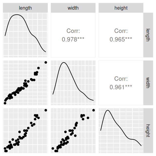
From Figure 7.2, it looks like all three of the variables are highly correlated and mostly reflect the same “underlying” variable, which we might interpret as the size of the turtle.
library("ComplexHeatmap")
mycolourscale = circlize::colorRamp2(c(-1, 0, 1), c("#FFD700", "#f0f0f0", "#0057B7"))
Heatmap(cor(athletes_1), col = mycolourscale, name = "Correlation")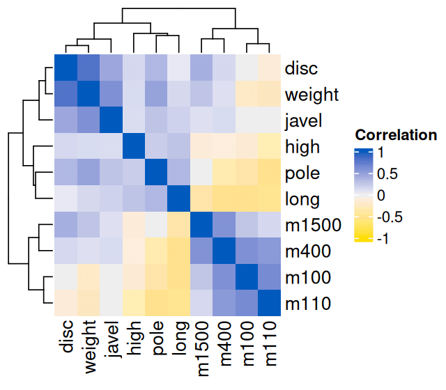
athletes_1 data. The hierarchical clustering shows a grouping of related disciplines.
Figure 7.3 shows how the 10 variables cluster into groups: running, throwing and jumping.
In many cases, different variables are measured in different units, so they have different baselines and different scales6. They are not directly comparable in their original form.
6 Common measures of scale are the range and the standard deviation. For instance, the times for the 110 metres vary between 14.18 and 16.2, with a standard deviation of 0.51, whereas the times to complete the 1500 metres vary between 256.64 and 303.17, with a standard deviation of 13.66; more than an order of magnitude larger. Moreover, the athletes_1 data also contain measurements in different units (seconds, metres), whose choice is arbitrary (lengths could also be recorded in centimetres or feet, times in milliseconds).
For PCA and many other methods, we therefore need to transform the numeric values to some common scale in order to make comparisons meaningful. Centering means subtracting the mean, so that the mean of the centered data is at the origin. Scaling or standardizing then means dividing by the standard deviation, so that the new standard deviation is \(1\). In fact, we have already encountered these operations when computing the correlation coefficient (Equation 7.1): the correlation coefficient is simply the vector product of the centered and scaled variables. To perform these operations, there is the R function scale, whose default behavior when given a matrix or a data frame is to make every column have a mean of zero and a standard deviation of \(1\).
apply(turtles[, -1], 2, sd)length width height
20.48 12.68 8.39 apply(turtles[, -1], 2, mean)length width height
124.7 95.4 46.3 scaledTurtles = scale(turtles[, -1])
apply(scaledTurtles, 2, mean) length width height
-1.43e-18 1.94e-17 -2.87e-16 apply(scaledTurtles, 2, sd)length width height
1 1 1 data.frame(scaledTurtles, sex = turtles[, 1]) %>%
ggplot(aes(x = width, y = height, group = sex)) +
geom_point(aes(color = sex)) +
coord_fixed()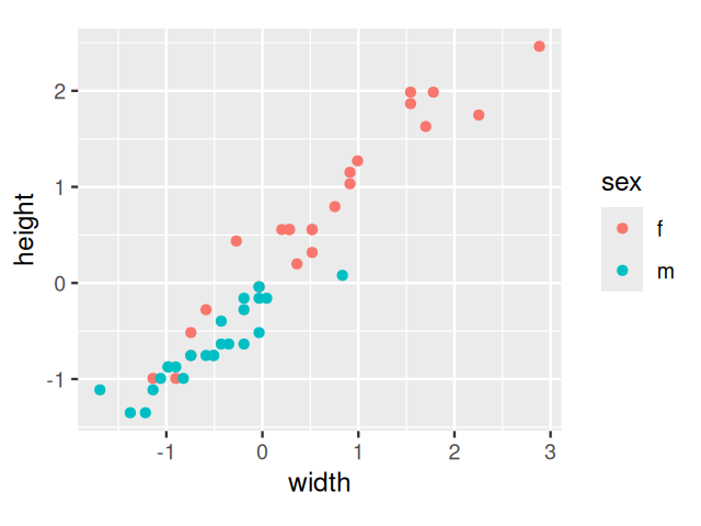
width and height variables: each point colored according to sex.
In Figure 7.3, we see an anticorrelation between the running disciplines (m100, m110, m400, m1500) and the jumping and throwing disciplines. This is due to the fact that better performances in running are associated with shorter times (smaller numeric values), whereas better performances in throwing and jumping lead to larger lengths (higher numeric values). We can address this by converting the time measurements into speed measurements (in m/s):
athletes_2 = mutate(athletes_1,
    m100 = 100 / m100,
    m110 = 110 / m110,
    m400 = 400 / m400,
    m1500 = 1500 / m1500
)
Let us then redo the plot:
library("ComplexHeatmap")
mycolourscale = circlize::colorRamp2(c(-1, 0, 1), c("#FFD700", "#f0f0f0", "#0057B7"))
Heatmap(cor(athletes_2), col = mycolourscale, name = "Correlation")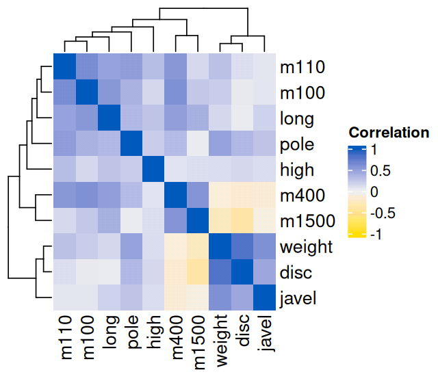
athletes_2 data. Compare to Figure 7.3.
We have already encountered other data transformation choices in Chapters 4 and 5, where we used the log and asinh functions. The aim of these transformations is (usually) variance stabilization, i.e., to make the variances of replicate measurements of one and the same variable in different parts of its dynamic range more similar. In contrast, the standardizing transformation described above aims to make the scale (as measured by mean and standard deviation) of different variables the same.
Sometimes it is preferable to leave variables at different scales because they are truly of different importance. If their original scale is relevant, then we can (should) leave the data as is. In other cases, the variables have different precisions known a priori. We will see in Chapter 9 that there are several ways of weighting such variables.
After preprocessing the data, we are ready to undertake data simplification through dimension reduction.
![]()
We will explain dimension reduction from several different perspectives. It was invented in 1901 by Karl Pearson (Pearson 1901) as a way to reduce a two-variable scatterplot to a single coordinate. It was used by statisticians in the 1930s to summarize a battery of psychological tests run on the same subjects (Hotelling 1933); thus providing overall scores that summarize many tested variables at once.
This idea of principal scores inspired the name Principal Component Analysis (abbreviated PCA). PCA is called an unsupervised learning technique because, as in clustering, it treats all variables as having the same status. We are not trying to predict or explain one particular variable’s value from the others; rather, we are trying to find a mathematical model for an underlying structure for all the variables. PCA is primarily an exploratory technique that produces maps that show the relations between variables and between observations in a useful way.
We first provide a flavor of what this multivariate analysis does to the data. There is an elegant mathematical formulation of these methods through linear algebra, although here we will try to minimize its use and focus on visualization and data examples.
We use geometrical projections that take points in higher-dimensional spaces and projects them down onto lower dimensions. Figure 7.6 shows the projection of the point \(A\) onto the line generated by the vector \({\mathbf v}\).
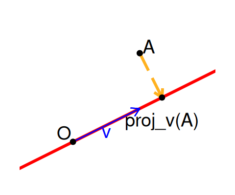
PCA is a linear technique, meaning that we look for linear relations between variables and that we will use new variables that are linear functions of the original ones (\(f(ax+by)=af(x)+b(y)\)). The linearity constraints makes computations particularly easy. We will see non-linear techniques in Chapter 9.
Here we show one way of projecting two-dimensional data onto a line using the athletes data. The code below provides the preprocessing and plotting steps that were used to generate Figure 7.7:
athletes_3 = data.frame(scale(athletes_2))
ath_gg = ggplot(athletes_3, aes(x = weight, y = disc)) +
  geom_point(size = 2, shape = 21)
ath_gg +
  geom_point(aes(y = 0), colour = "red") +
  geom_segment(aes(xend = weight, yend = 0), linetype = "dashed")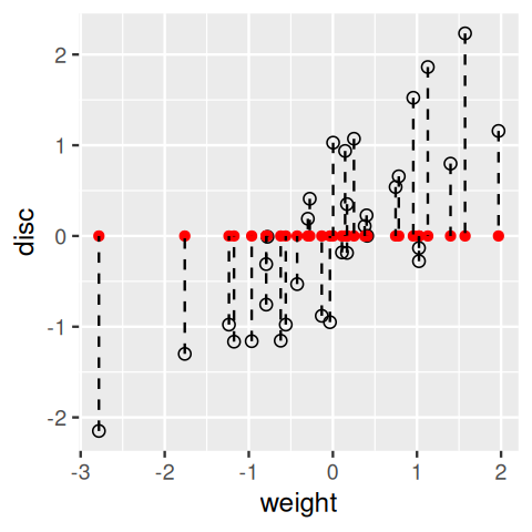
In general, we lose information about the points when we project from two dimensions (a plane) to one (a line). If we do it just by using the original coordinates, as we did on the weight variable in Figure 7.7, we lose all the information about the disc variable. Our goal is to keep as much information as we can about both variables. There are actually many ways of projecting the point cloud onto a line. One is to use what are known as regression lines. Let’s look at these lines and how they are constructed in R.
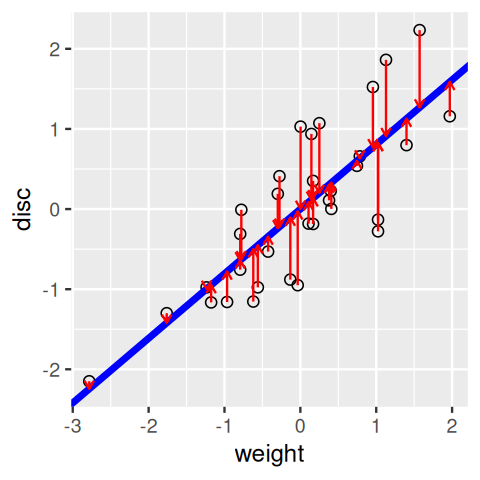
If you have seen linear regression, you already know how to compute lines that summarize scatterplots; linear regression is a supervised method that gives preference minimizing the residual sum of squares in one direction: that of the response variable.
disc variable on weight.In Figure 7.8, we use the lm (linear model) function to find the regression line. Its slope and intercept are given by the values in the coefficients slot of the resulting object reg1.
reg1 = lm(disc ~ weight, data = athletes_3)
a1 = reg1$coefficients[1] # intercept
b1 = reg1$coefficients[2] # slope
pline1 = ath_gg +
  geom_abline(intercept = a1, slope = b1, col = "blue", linewidth = 1.5)
pline1 +
  geom_segment(
    aes(xend = weight, yend = reg1$fitted.values),
    colour = "red",
    arrow = arrow(length = unit(0.15, "cm"))
  )
weight on discus.Figure 7.9 shows the line produced when reversing the roles of the two variables; weight becomes the response variable.
reg2 = lm(weight ~ disc, data = athletes_3)
a2 = reg2$coefficients[1] # intercept
b2 = reg2$coefficients[2] # slope
pline2 = ath_gg +
  geom_abline(
    intercept = -a2 / b2,
    slope = 1 / b2,
    col = "darkgreen",
    linewidth = 1.5
  )
pline2 +
  geom_segment(
    aes(xend = reg2$fitted.values, yend = disc),
    colour = "orange",
    arrow = arrow(length = unit(0.15, "cm"))
  )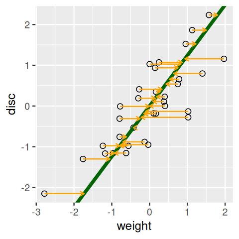
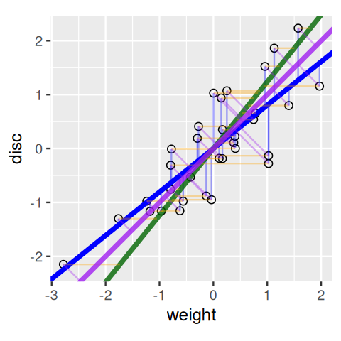
Each of the regression lines in Figures 7.8 and 7.9 gives us an approximate linear relationship between disc and weight. However, the relationship differs depending on which of the variables we choose to be the predictor and which the response.
Figure 7.10 shows the line chosen to minimize the sum of squares of the orthogonal (perpendicular) projections of data points onto it; we call this the principal component line. All our three ways of fitting a line (Figures 7.8–7.10) together in one plot are shown in Figure 7.11.
xy = with(athletes_3, cbind(disc, weight))
svda = svd(xy)
pc = xy %*% svda$v[, 1] %*% t(svda$v[, 1])
bp = svda$v[2, 1] / svda$v[1, 1]
ap = mean(pc[, 2]) - bp * mean(pc[, 1])
ath_gg +
  geom_segment(xend = pc[, 1], yend = pc[, 2]) +
  geom_abline(intercept = ap, slope = bp, col = "purple", linewidth = 1.5)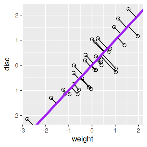
Pythagoras’ theorem tells us two interesting things here:
If we are minimizing in both horizontal and vertical directions we are in fact minimizing the orthogonal projections onto the line from each point.
The total variability of the points is measured by the sum of squares of the projection of the points onto the center of gravity, which is the origin (0,0) if the data are centered. This is called the total variance or the inertia of the point cloud. This inertia can be decomposed into the sum of the squares of the projections onto the line plus the variances along that line. For a fixed variance, minimizing the projection distances also maximizes the variance along that line. Often we define the first principal component as the line with maximum variance.

The PC line we found in the previous section could be written
\[ PC = \frac{1}{2} \mbox{disc} + \frac{1}{2} \mbox{weight}. \tag{7.2}\]
Principal components are linear combinations of the variables that were originally measured, they provide a new coordinate system. To understand what a linear combination really is, we can take an analogy. When making a healthy juice mix, you will follow a recipe like
\[ \begin{align} V &= 2 \times \text{Beet} + 1 \times \text{Carrot} \\ &+ \tfrac{1}{2} \text{Gala} + \tfrac{1}{2} \text{GrannySmith} \\ &+ 0.02 \times \text{Ginger} + 0.25 \times \text{Lemon}. \end{align} \]
This recipe is a linear combination of individual juice types (the original variables). The result is a new variable, \(V\), and the coefficients \((2,1,\frac{1}{2},\frac{1}{2},0.02,0.25)\) are called the loadings.
A linear combination of variables defines a line in higher dimensions in the same way we constructed lines in the scatterplot plane of two dimensions. As we saw in that case, there are many ways to choose lines onto which we project the data, there is however a `best’ line for our purpose.
The total variance of all the points in all the variables can de decomposed. In PCA, we use the fact that the total sums of squares of the distances between the points and any line can be decomposed into the distance to the line and the variance along the line.
We saw that the principal component minimizes the distance to the line, and it also maximizes the variance of the projections along the line.
Why is maximizing the variance along a line a good idea? Let’s look at another example of a projection from three dimensions into two. In fact, human vision depends on such dimension reduction:

PCA is based on the principle of finding the axis showing the largest inertia/variability, removing the variability in that direction and then iterating to find the next best orthogonal axis, and so on. In fact, we do not have to run iterations, all the axes can be found in one linear algebra operation called the Singular Value Decomposition (we will delve more deeply into the details below).
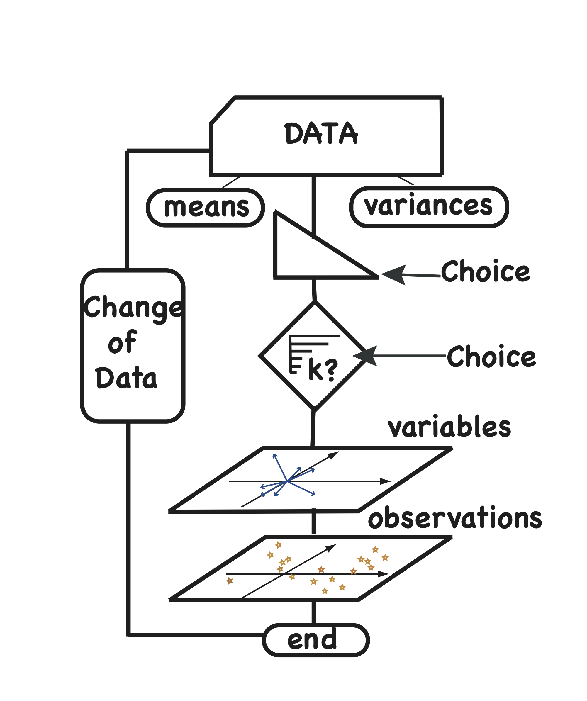
In the diagram in Figure 7.13, we see that first the means and variances are computed and the choice of whether to work directly with the covariance matrix or with the correlation matrix has to be made. The next step is the choice of \(k\), the number of components we deem relevant to the data. We say that \(k\) is the rank of the approximation. The best choice of \(k\) is a difficult question, and we discuss on how to approach it below. The choice of \(k\) requires looking at a plot of the variances explained by the successive principal components. Once we have chosen \(k\), we can proceed to the projections of the data in the new \(k\)-dimensional subspace.
The end results of the PCA workflow are useful maps of both the variables and the samples. Understanding how these maps are constructed will maximize the information we can gather from them.
This is a small section for those whose background in linear algebra is but a faint memory. It tries to give some intuition to the singular value decomposition method underlying PCA, without too much notation.

The singular value decomposition of a matrix finds horizontal and vertical vectors (called the singular vectors) and normalizing values (called singular values). As before, we start by giving the forward-generative explanation before doing the actual reverse engineering that is used in creating the decomposition. To calibrate the meaning of each step, we will start with an artificial example before moving to the complexity of real data.
A simple generative model demonstrates the meaning of the rank of a matrix and explains how we find it in practice. Suppose we have two vectors, \(u\) (a one-column matrix), and \(v^t=t(v)\) (a one-row matrix–the transpose of a one-column matrix \(v\)). For instance, \(u =\left( \begin{smallmatrix} 1\\2\\3\\4 \end{smallmatrix} \right)\) and \(v =\left( \begin{smallmatrix} 2\\4\\8 \end{smallmatrix} \right)\). The transpose of \(v\) is written \(v^t = t(v) = (2\; 4\; 8)\). We multiply a copy of \(u\) by each of the elements of \(v^t\) in turn as follows:
Step 0:
| X | 2 | 4 | 8 |
|---|---|---|---|
| 1 | |||
| 2 | |||
| 3 | |||
| 4 |
Step 1:
| X | 2 | 4 | 8 |
|---|---|---|---|
| 1 | 2 | ||
| 2 | 4 | ||
| 3 | 6 | ||
| 4 | 8 |
Step 2:
| X | 2 | 4 | 8 |
|---|---|---|---|
| 1 | 2 | 4 | |
| 2 | 4 | 8 | |
| 3 | 6 | 12 | |
| 4 | 8 | 16 |
Step 3:
| X | 2 | 4 | 8 |
|---|---|---|---|
| 1 | 2 | 4 | 8 |
| 2 | 4 | 8 | 16 |
| 3 | 6 | 12 | 24 |
| 4 | 8 | 16 | 32 |
Thus, the \((2,3)\) entry of the matrix \(X\), written \(x_{2,3}\), is obtained by multiplying \(u_2\) by \(v_3\). We can write this
\[ X=\begin{pmatrix} 2&4&8\\ 4&8&16\\ 6 &12&24\\ 8&16&32\\ \end{pmatrix} = u * t(v)= u * v^t \tag{7.3}\]
The matrix \(X\) we obtain here is said to be of rank 1, because both \(u\) and \(v\) have one column.
On the other hand, suppose that we want to reverse the process and simplify another matrix \(X\) given below with 3 rows and 4 columns (12 numbers). Can we always express it in a similar way as a product of vectors without loss of information? In the diagrams shown in Figures 7.15 and 7.16, the colored boxes have areas proportional to the numbers in the cells of the matrix (7.4).
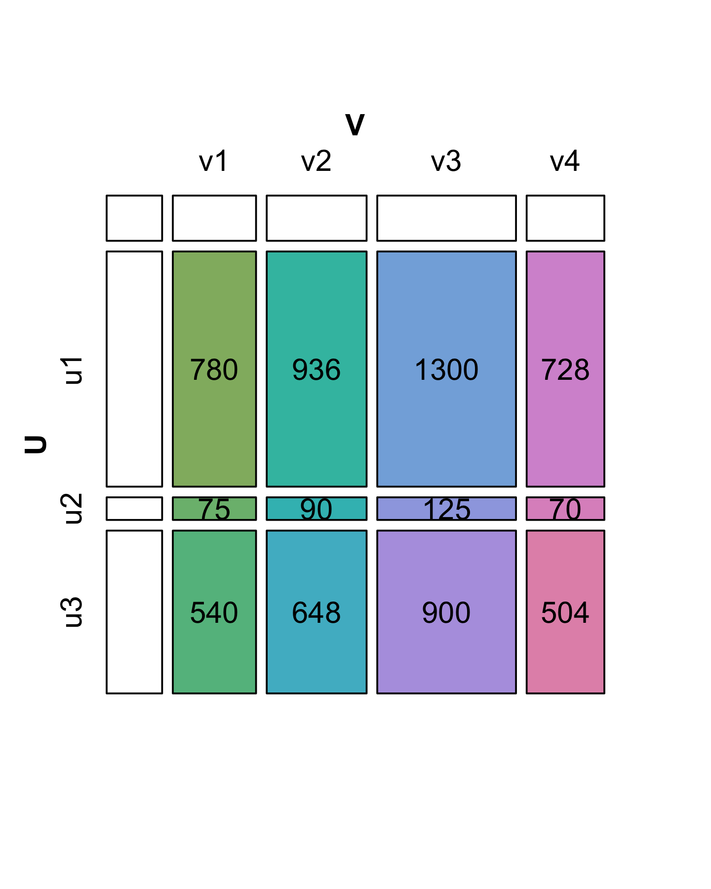
A matrix with the special property of being perfectly “rectangular” like \(X\) is said to be of rank 1. We can represent the numbers in \(X\) by the areas of rectangles, where the sides of rectangles are given by the values in the side vectors (\(u\) and \(v\)).
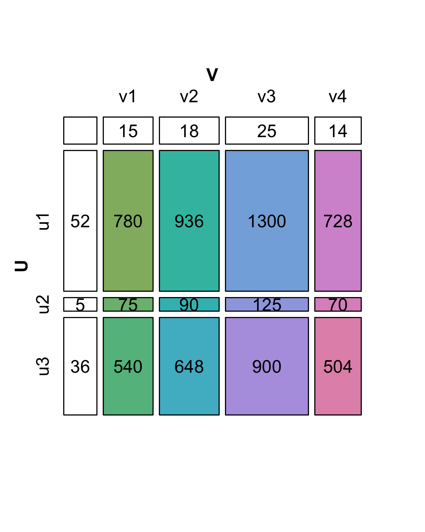

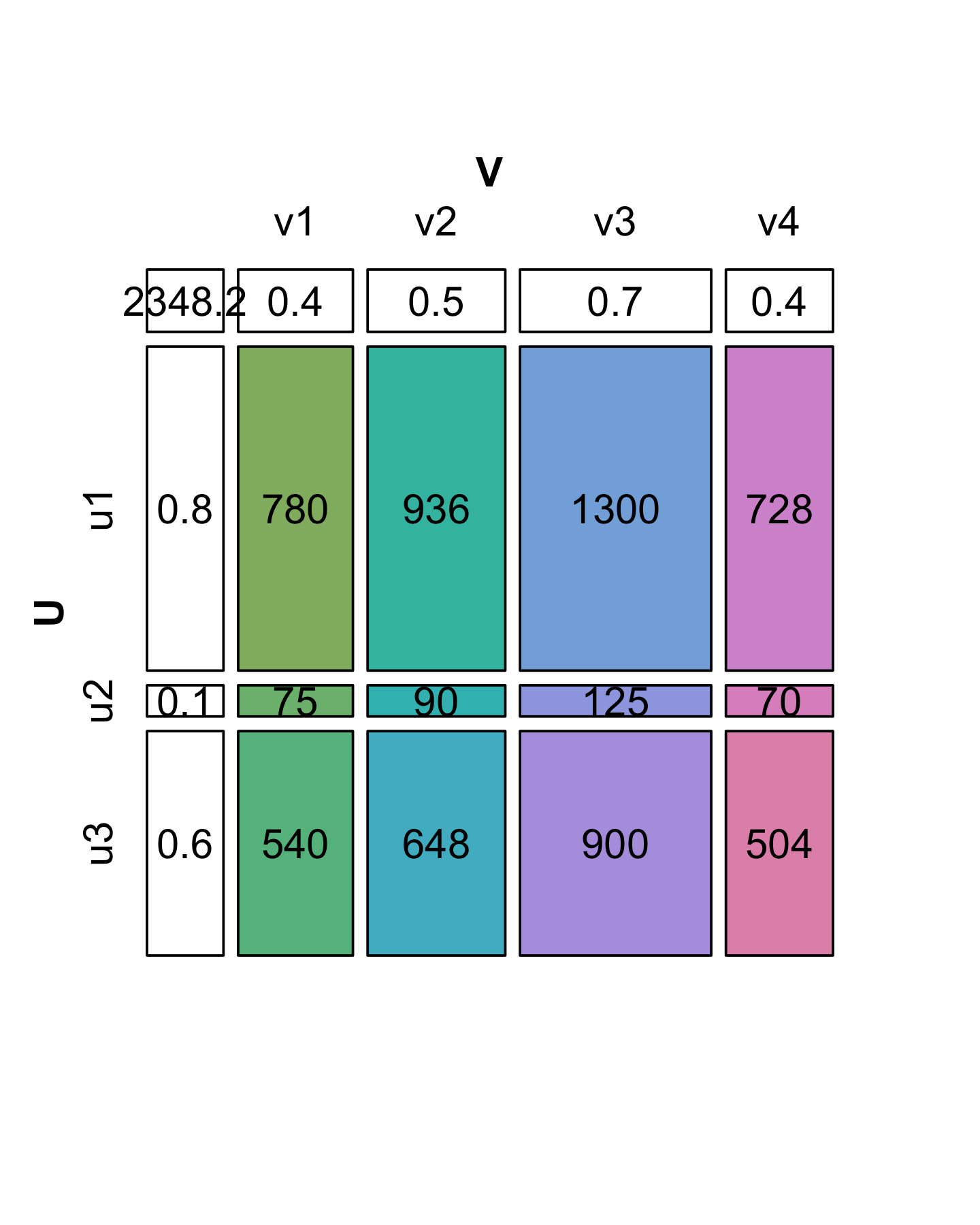
We see in Figure 7.16 that the decomposition of \(X\) is not unique: there are several candidate choices for the vectors \(u\) and \(v\). We will make the choice unique by requiring that the sum of the squares of each vector’s elements add to 1 (we say the vectors \(v\) and \(u\) have norm 1). Then we have to keep track of one extra number by which to multiply each of the products, and which represents the “overall scale” of \(X\). This is the value we have put in the upper left hand corner. It is called the singular value \(s_1\). In the R code below, we start by supposing we know the values in u, v and s1; later we will see a function that finds them for us. Let’s check the multiplication and norm properties in R:
u = c(0.8196, 0.0788, 0.5674)
v = c(0.4053, 0.4863, 0.6754, 0.3782)
s1 = 2348.2
sum(u^2)
[1] 1sum(v^2)[1] 1s1 * u %*% t(v) [,1] [,2] [,3] [,4]
[1,] 780 936 1300 728
[2,] 75 90 125 70
[3,] 540 648 900 504X - s1 * u %*% t(v) [,1] [,2] [,3] [,4]
[1,] -0.03419 0.0745 0.1355 0.1221
[2,] 0.00403 0.0159 0.0252 0.0186
[3,] -0.00903 0.0691 0.1182 0.0982In fact, in this particular case we were lucky: we see that the second and third singular values are 0 (up to the numeric precision we care about). That is why we say that \(X\) is of rank 1. For a more general matrix \(X\), it is rare to be able to write \(X\) exactly as this type of two-vector product. The next subsection shows how we can decompose \(X\) when it is not of rank 1: we will just need more pieces.
In the above decomposition, there were three elements: the horizontal and vertical singular vectors, and the diagonal corner, called the singular value. These can be found using the singular value decomposition function (svd). For instance:
Xtwo = matrix(c(
    12.5, 35,   25, 25,
     9  , 14,   26, 18,
    16. , 21,   49, 32,
    18. , 28,   52, 36,
    18, 10.5, 64.5, 36),
  ncol = 4,
  byrow = TRUE)
USV = svd(Xtwo)Again, there are many ways to write a rank two matrix such as Xtwo as a sum of rank one matrices: in order to ensure uniqueness, we impose yet another7 condition on the singular vectors. The output vectors of the singular decomposition do not only have their norms equal to 1, each column vector in the \(U\) matrix is orthogonal to all the previous ones. We write \(u_{\cdot 1} \perp u_{\cdot 2}\), this means that the sum of the products of the values in the same positions is \(0\): \(\sum_i u_{i1} u_{i2} = 0\). Ditto for the \(V\) matrix.
7 Above, we had chosen the norm of the vectors to be 1.
Let’s submit our scaledTurtles matrix to a singular value decomposition.
turtles.svd = svd(scaledTurtles)
turtles.svd$d
[1] 11.75 1.42 1.00turtles.svd$v [,1] [,2] [,3]
[1,] 0.579 0.325 0.748
[2,] 0.578 0.483 -0.657
[3,] 0.575 -0.813 -0.092dim(turtles.svd$u)[1] 48 3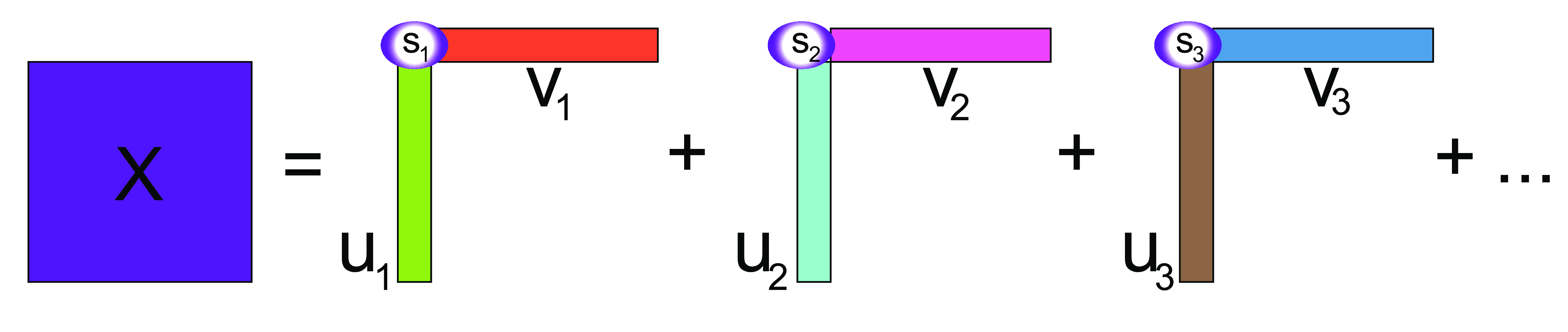
\(X\) is decomposed additively into rank-one pieces. Each of the \(u\) vectors is combined into the \(U\) matrix, and each of \(v\) vectors into \(V\). The Singular Value Decomposition is
\[ {\mathbf X} = U S V^t, V^t V={\mathbb I}, U^t U={\mathbb I}, \tag{7.5}\]
where \(S\) is the diagonal matrix of singular values, \(V^t\) is the transpose of \(V\), and \({\mathbb I}\) is the Identity matrix. Expression 7.5 can be written elementwise as
\[ X_{ij} = u_{i1}s_1v_{1j} + u_{i2}s_2v_{2j} + u_{i3}s_3v_{3j} +... + u_{ir}s_rv_{rj}, \]
\(U\) and \(V\) are said to be orthonormal8, because their self-crossproducts are the identity matrix.
8 Nothing to do with the normal distribution, it stands for orthogonal and having norm 1.
The singular vectors from the singular value decomposition (provided by the svd function in R) contain the coefficients to put in front of the original variables to make the more informative ones we call the principal components. We write this as:
\[ Z_1=v_{11} X_{\cdot 1} +v_{21} X_{\cdot 2} + v_{31} X_{\cdot 3}+ \cdots + v_{p1} X_{\cdot p}. \]
If usv = svd(X), then \((v_{11},v_{21},v_{31},...)\) are given by the first column of usv$v; similarly for \(Z_2\) with the second column of usv$v, and so son. \(p\) is the number of columns of \(X\) and the number of rows of \(V\). These new variables \(Z_1, Z_2, Z_3, ...\) have variances that decrease in size: \(s_1^2 \geq s_2^2 \geq s_3^2 \geq ...\).
Here are two useful facts, first in words, then with the mathematical shorthand.
The number of principal components \(k\) is always chosen to be fewer than the number of original variables or the number of observations. We are “lowering” the dimension of the problem:
\[ k\leq \min(n,p). \]
The principal component transformation is defined so that the first principal component has the largest possible variance (that is, accounts for as much of the variability in the data as possible), and each successive component in turn has the highest variance possible under the constraint that it be orthogonal to the preceding components:
\[ \max_{aX \perp bX}\mbox{var}(\mbox{Proj}_{aX} (X)), \qquad \mbox{where } bX=\mbox{previous components} \]
We revisit our two-variable athletes data with the discus and the weight variables. In Section 7.3.2, we computed the first principal component and represented it as the purple line in Figure 7.11. We showed that \(Z_1\) was the linear combination given by the diagonal. As the coefficients have to have their sum of squares add to \(1\), we have that \[Z_1=-0.707*\text{athletes\$disc}- 0.707*\text{athletes\$weight}.\]
svda which was the svd applied to the two variables discus and weight.If we rotate the (discus, weight) plane by making the purple line the horizontal \(x\) axis, we obtain what is know as the first principal plane.
ppdf = tibble(PC1n = -svda$u[, 1] * svda$d[1], PC2n = svda$u[, 2] * svda$d[2])
gg = ggplot(ppdf, aes(x = PC1n, y = PC2n)) +
geom_point() +
geom_hline(yintercept = 0, color = "purple", linewidth = 1.5, alpha = 0.5) +
xlab("PC1 ") +
ylab("PC2") +
xlim(-3.5, 2.7) +
ylim(-2, 2) +
coord_fixed()
gg +
geom_point(aes(x = PC1n, y = 0), color = "red") +
geom_segment(aes(xend = PC1n, yend = 0), color = "red")
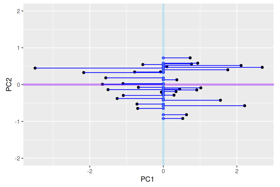
gg +
geom_point(aes(x = 0, y = PC2n), color = "blue") +
geom_segment(aes(yend = PC2n, xend = 0), color = "blue") +
geom_vline(xintercept = 0, color = "skyblue", linewidth = 1.5, alpha = 0.5)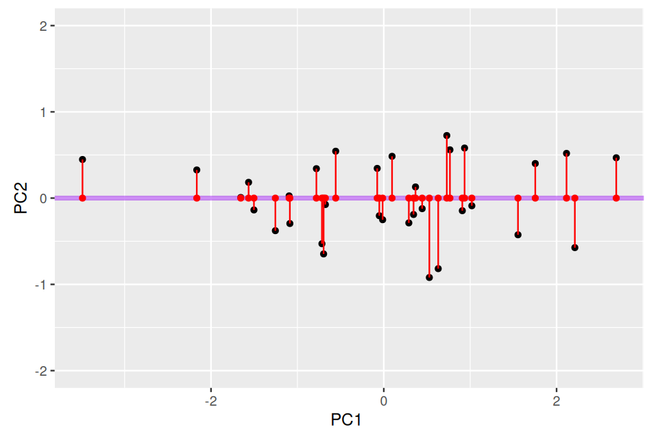
We now want to do a complete PCA analysis on the turtles data. Remember, we already looked at the summary statistics for the one- and two-dimensional data. Now we are going to answer the question about the “true” dimensionality of these rescaled data.
In the following code, we use the function princomp. Its return value is a list of all the important pieces of information needed to plot and interpret a PCA.
cor(scaledTurtles) length width height
length 1.000 0.978 0.965
width 0.978 1.000 0.961
height 0.965 0.961 1.000pcaturtles = princomp(scaledTurtles)
pcaturtlesCall:
princomp(x = scaledTurtles)
Standard deviations:
Comp.1 Comp.2 Comp.3
1.695 0.205 0.145
3 variables and 48 observations.library("factoextra")
fviz_eig(pcaturtles, geom = "bar", bar_width = 0.4) + ggtitle("")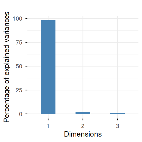
scaledTurtles): there is one large value and two small ones. The data are (almost) one-dimensional. We will see why this dimension is called an axis of size, a frequent phenomenon in biometric data (Jolicoeur and Mosimann 1960).
In what follows, we always suppose that the matrix \(X\) represents the centered and scaled matrix.
Now we are going to combine both the PC scores (\(US\)) and the loadings-coefficients (\(V\)). The plots with both the samples and the variables represented are called biplots. This can be done in one line using the following factoextra package function.
# See https://github.com/kassambara/ggpubr/issues/645
#| warning.known: !expr c("Using `size` aesthetic for lines was deprecated in ggplot2 3.4.0.")
#| fig-width: 6
#| fig-height: 2
#| fig-margin: false
#| fig-cap-location: margin
#| fig-cap: "A biplot of the first two dimensions showing both variables and observations. The arrows show the variables. The turtles are labeled by sex. The extended horizontal direction is due to the size of the first eigenvalue, which is much larger than the second."
fviz_pca_biplot(pcaturtles, label = "var", habillage = turtles[, 1]) +
  ggtitle("")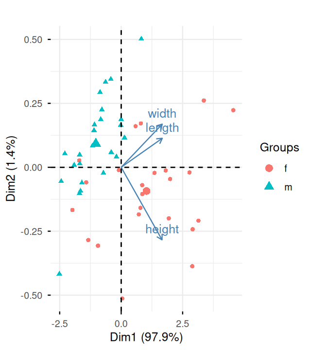
Now we look at the relationships between the variables, both old and new by drawing what is known as the correlation circle. The aspect ratio is 1 here and the variables are represented by arrows as shown in Figure 7.20. The lengths of the arrows indicate the quality of the projections onto the first principal plane:
fviz_pca_var(pcaturtles, col.circle = "black") +
  ggtitle("") +
  xlim(c(-1.2, 1.2)) +
  ylim(c(-1.2, 1.2))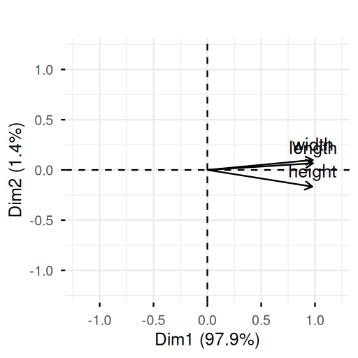
These data are a good example of how sometimes almost all the variation in the data can be captured in a lower-dimensional space: here, three-dimensional data can be essentially replaced by a line. Keep in mind: \(X^tC=VSU^tUS=VS^2.\) The principal components are the columns of the matrix \(C=US\). The \(p\) columns of \(U\) (the matrix given as USV$u in the output from the svd function above) are rescaled to have norms \((s_1^2,s_2^2,...,s_p^2)\). Each column has a different variance it is responsible for explaining. Notice that these will be decreasing numbers.
If the matrix \(X\) comes from the study of \(n\) different samples or specimens, then the principal components provides new coordinates for these \(n\) points as in Figure 7.17. These are sometimes called the scores in the results of PCA functions.
Before we go into more detailed examples, let’s summarize what SVD and PCA provide:
Each principal component has a variance measured by the corresponding eigenvalue, the square of the corresponding singular value.
The new variables are made to be orthogonal. Since they are also centered, this means they are uncorrelated. In the case of normal distributed data, this also means they are independent.
When the variables are have been rescaled, the sum of the variances of all the variables is the number of variables (\(=p\)). The sum of the variances is computed by adding the diagonal of the crossproduct matrix9.
The principal components are ordered by the size of their eigenvalues. We always check the screeplot before deciding how many components to retain. It is also best practice to do as we did in Figure 7.19 and annotate each PC axis with the proportion of variance it explains.
9 This sum of the diagonal elements is called the trace of the matrix.
![]()
We started looking at these data earlier in this chapter. Here, we will follow step by step a complete multivariate analysis. First, let us have another look at the correlation matrix, which captures the bivariate associations. We already plotted it as a colored heatmap in Figure 7.5.
cor(athletes_3) m100 long weight high m400 m110 disc pole javel m1500
m100 1.0000 0.5406 0.2099 0.143 0.5951 0.636 0.0495 0.3852 0.0670 0.2442
long 0.5406 1.0000 0.1419 0.273 0.5106 0.481 0.0419 0.3499 0.1817 0.3914
weight 0.2099 0.1419 1.0000 0.122 -0.0972 0.292 0.8064 0.4800 0.5977 -0.2686
high 0.1428 0.2731 0.1221 1.000 0.0850 0.307 0.1474 0.2132 0.1159 0.1066
m400 0.5951 0.5106 -0.0972 0.085 1.0000 0.538 -0.1386 0.3175 -0.1197 0.5819
m110 0.6361 0.4811 0.2921 0.307 0.5383 1.000 0.1091 0.5252 0.0700 0.1320
disc 0.0495 0.0419 0.8064 0.147 -0.1386 0.109 1.0000 0.3440 0.4429 -0.3970
pole 0.3852 0.3499 0.4800 0.213 0.3175 0.525 0.3440 1.0000 0.2742 0.0369
javel 0.0670 0.1817 0.5977 0.116 -0.1197 0.070 0.4429 0.2742 1.0000 -0.0887
m1500 0.2442 0.3914 -0.2686 0.107 0.5819 0.132 -0.3970 0.0369 -0.0887 1.0000Then we look at the screeplot, which will help us choose a rank \(k\) for representing the essence of these data.
pca.ath = dudi.pca(athletes_3, scannf = FALSE)
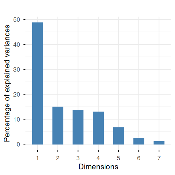
pca.ath$eig [1] 3.408 2.593 0.943 0.886 0.570 0.496 0.427 0.306 0.268 0.104fviz_eig(pca.ath, geom = "bar", bar_width = 0.3) + ggtitle("")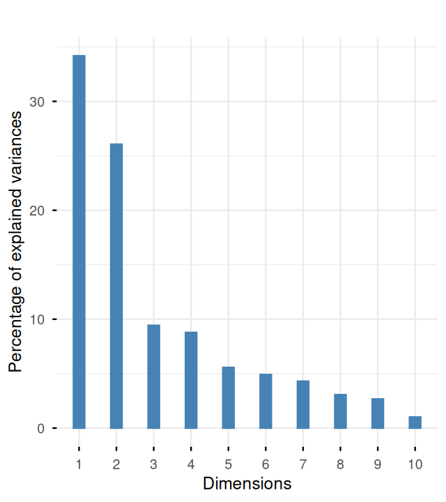
The screeplot in Figure 7.22 shows a clear drop in the eigenvalues after the second one. This indicates that a good approximation will be obtained at rank 2. Let’s look at an interpretation of the first two axes by projecting the loadings of the original variables onto the two new ones, the principal components.
fviz_pca_var(pca.ath, col.var = "blue", repel = TRUE) + ggtitle("")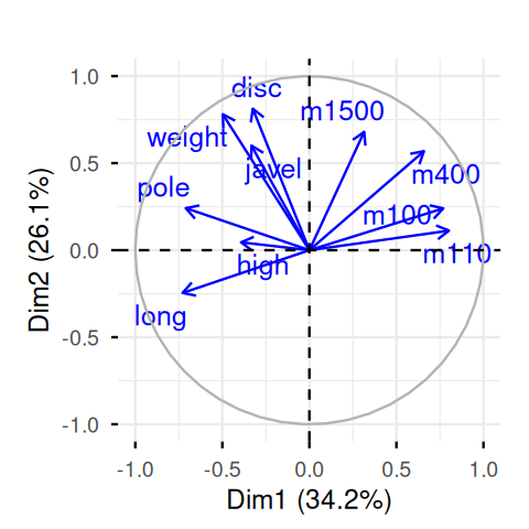
fviz_pca_ind(pca.ath, repel = TRUE) + ggtitle("")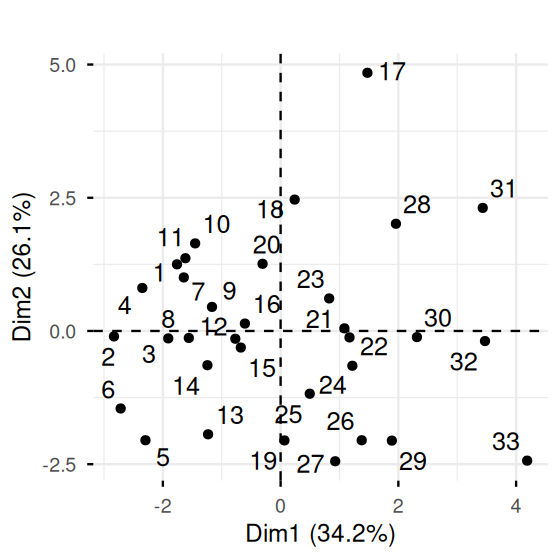
It turns out there is complementary information available in the olympic dataset. An extra vector variable called score reports the final scores at the competition, the men’s decathlon at the 1988 Olympics.
olympic$score [1] 8488 8399 8328 8306 8286 8272 8216 8189 8180 8167 8143 8114 8093 8083 8036
[16] 8021 7869 7860 7859 7781 7753 7745 7743 7623 7579 7517 7505 7422 7310 7237
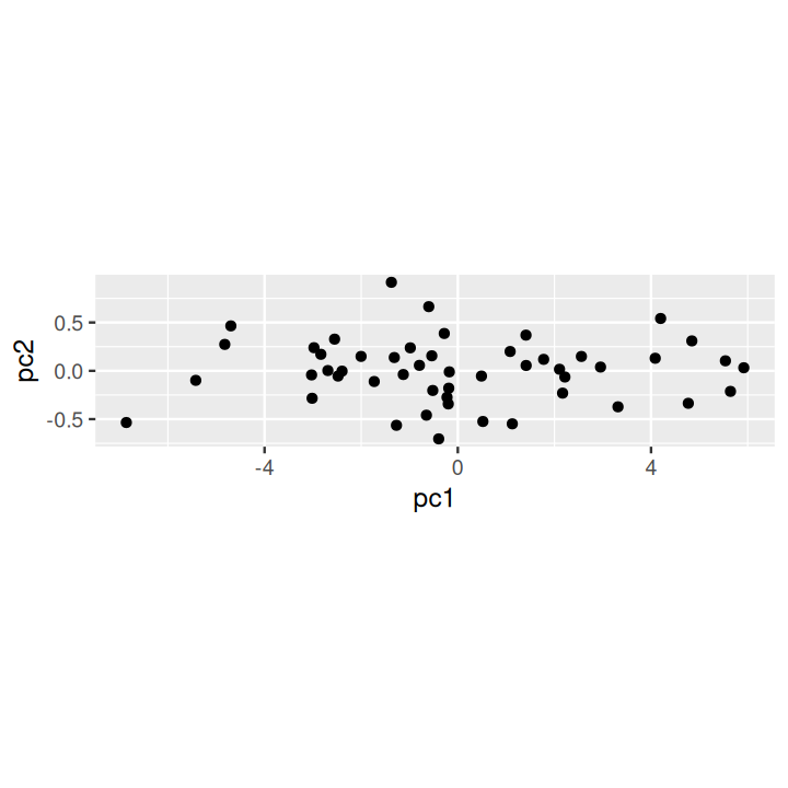
[31] 7231 7016 6907So let us look at the scatterplot comparing the first principal component coordinate of the athletes to this score. This is shown in Figure 7.25. We can see a strong correlation between the two variables. We note that athlete number 1 (who in fact won the Olympic decathlon gold medal) has the highest score, but not the highest value in PC1. Why do you think that is?
ggplot(
  data = tibble(
    pc1 = pca.ath$li[, 1],
    score = olympic$score,
    label = rownames(athletes_3)
  ),
  mapping = aes(y = score, x = pc1)
) +
  geom_text(aes(label = label)) +
  stat_smooth(method = "lm", se = FALSE)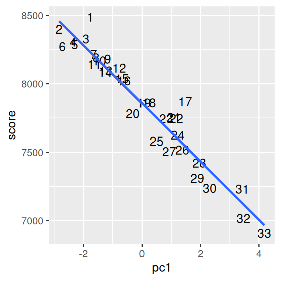
olympic$score and the first principal component. The points are labeled by their order in the data set. We can see a strong correlation. Why is it not a perfectly linear fit?
We have seen in the examples that the first step in PCA is to make the screeplot of the variances of the new variables (equal to the eigenvalues). We cannot decide how many dimensions are needed before seeing this plot. The reason is that there are situations when the principal components are ill-defined: when two or three successive PCs have very similar variances, giving a screeplot as in Figure 7.26, the subspace corresponding to a group of similar eigenvalues exists. In this case this would be 3D space generated by \(u_2,u_3,u_4\). The vectors are not meaningful individually and one cannot interpret their loadings. This is because a very slight change in one observations could give a completely different set of three vectors. These would generate the same 3D space, but could have very different loadings. We say the PCs are unstable.
We have seen that unlike regression, PCA treats all variables equally (to the extent that they were preprocessed to have equivalent standard deviations). However, it is still possible to map other continuous variables or categorical factors onto the plots in order to help interpret the results. Often we have complementary information on the samples, for example, diagnostic labels in the diabetes data or the cell types in the T-cell gene expression data.
Here we see how we can use such extra variables to inform our interpretation. The best place to store such so-called metadata is in appropriate slots of the data object (such as in the Bioconductor SummarizedExperiment class); the second-best, in additional columns of the data frame that also contains the numeric data. In practice, such information is often stored in a more or less cryptic manner in the row names of the matrix. Below, we need to face the latter scenario, and we use substr gymnastics to extract the cell types and show the screeplot in Figure 7.27 and the PCA in Figure 7.28.
pcaMsig3 = dudi.pca(
  Msig3transp,
  center = TRUE,
  scale = TRUE,
  scannf = FALSE,
  nf = 4
)
fviz_screeplot(pcaMsig3) + ggtitle("")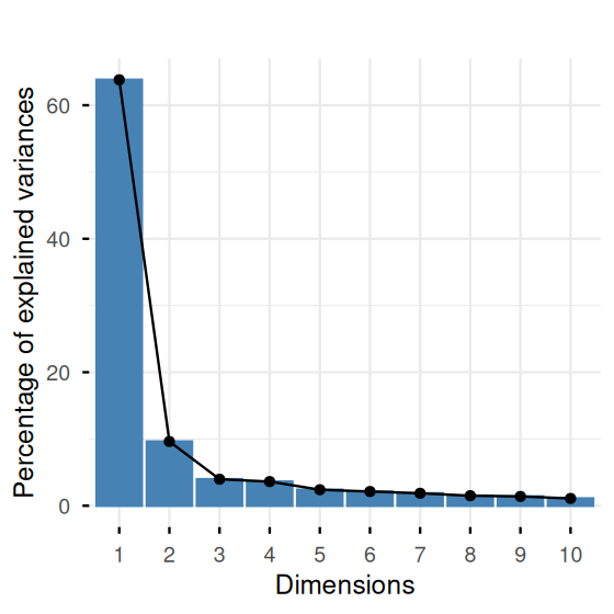
ids = rownames(Msig3transp)
celltypes = factor(substr(ids, 7, 9))
status = factor(substr(ids, 1, 3))
table(celltypes)
celltypes
EFF MEM NAI
10 9 11 cbind(pcaMsig3$li, tibble(Cluster = celltypes, sample = ids)) %>%
ggplot(aes(x = Axis1, y = Axis2)) +
geom_point(aes(color = Cluster), size = 5) +
geom_hline(yintercept = 0, linetype = 2) +
geom_vline(xintercept = 0, linetype = 2) +
scale_color_discrete(name = "Cluster") +
coord_fixed()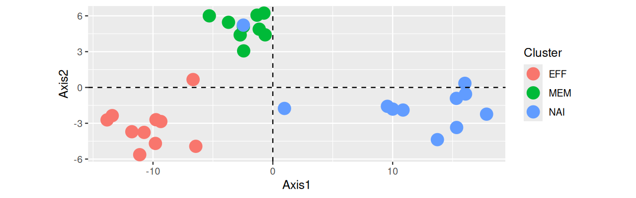
These data requires delicate preprocessing before we obtain our desired matrix with the relevant features as columns and the samples as rows. Starting with the raw mass spectroscopy readings, the steps involve extracting peaks of relevant features, aligning them across multiple samples and estimating peak heights. We refer the reader to the vignette of the Bioconductor xcms package for gruesome details. We load a matrix of data generated in such a way from the file mat1xcms.RData. The output of the below code is in Figures 7.29 and 7.30.
load("../data/mat1xcms.RData")
dim(mat1)
[1] 399 12pcamat1 = dudi.pca(t(mat1), scannf = FALSE, nf = 3)
fviz_eig(pcamat1, geom = "bar", bar_width = 0.7) + ggtitle("")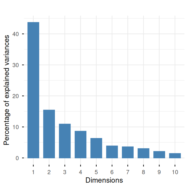
dfmat1 = cbind(
  pcamat1$li,
  tibble(
    label = rownames(pcamat1$li),
    number = substr(label, 3, 4),
    type = factor(substr(label, 1, 2))
  )
)
pcsplot = ggplot(
  dfmat1,
  aes(x = Axis1, y = Axis2, label = label, group = number, colour = type)
) +
  geom_text(size = 4, vjust = -0.5) +
  geom_point(size = 3) +
  ylim(c(-18, 19))
pcsplot +
  geom_hline(yintercept = 0, linetype = 2) +
  geom_vline(xintercept = 0, linetype = 2)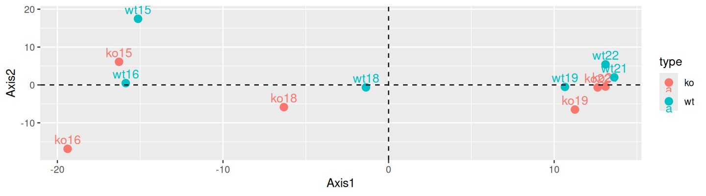
mat1 data. It explains 59% of the variance.
In the previous example, the number of variables measured was too large to enable useful concurrent plotting of both variables and samples. In this example we plot the PCA biplot of a simple data set where chemical measurements were made on different wines for which we also have a categorical wine.class variable. We start the analysis by looking at the two-dimensional correlations and a heatmap of the variables.
library("pheatmap")
load("../data/wine.RData")
load("../data/wineClass.RData")
wine[1:2, 1:7]
Alcohol MalicAcid Ash AlcAsh Mg Phenols Flav
1 14.2 1.71 2.43 15.6 127 2.80 3.06
2 13.2 1.78 2.14 11.2 100 2.65 2.76pheatmap(1 - cor(wine), treeheight_row = 0.2)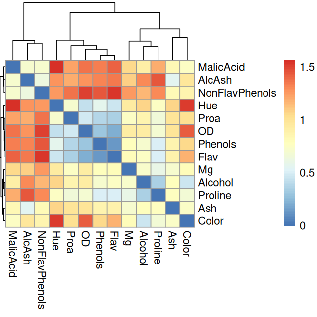
A biplot is a simultaneous representation of both the space of observations and the space of variables. In the case of a PCA biplot like Figure 7.32 the arrows represent the directions of the old variables as they project onto the plane defined by the first two new axes. Here the observations are just colored dots, the color has been chosen according to which type of wine is being plotted. We can interpret the variables’ directions with regards to the sample points, for instance the blue points are from the barbera group and show higher Malic Acid content than the other wines.
winePCAd = dudi.pca(wine, scannf = FALSE)
table(wine.class)
wine.class
barolo grignolino barbera
59 71 48 fviz_pca_biplot(
winePCAd,
geom = "point",
habillage = wine.class,
col.var = "violet",
addEllipses = TRUE,
ellipse.level = 0.69
) +
ggtitle("") +
coord_fixed()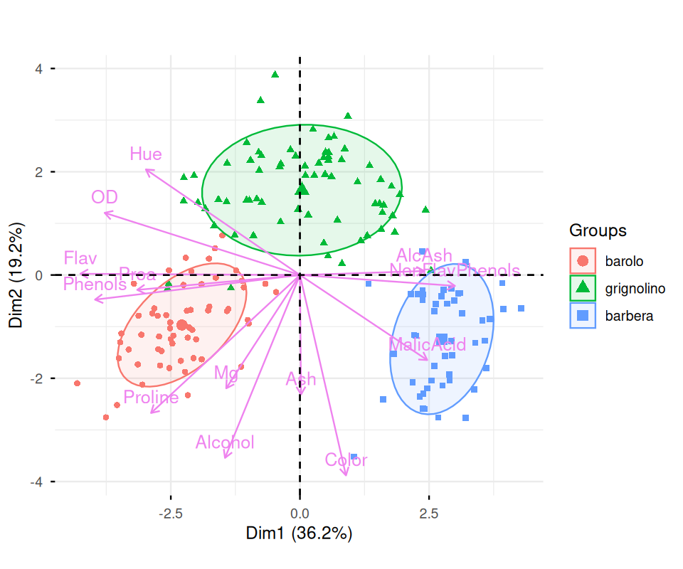
Phenols, Flav and Proa indicate that they are strongly correlated, whereas Hue and Alcohol are uncorrelated.
Interpretation of multivariate plots requires the use of as much of the available information as possible; here we have used the samples and their groups as well as the variables to understand the main differences between the wines.
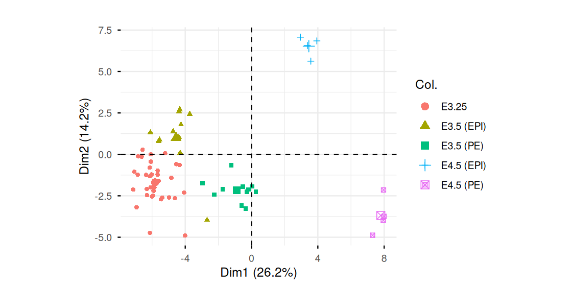
Sometimes we want to see variability between different groups or observations, but want to weight them. This can be the case if, e.g., the groups have very different sizes. Let’s re-examine the Hiiragi data we already saw in Chapter 3. In the code below, we select the wildtype (WT) samples and the top 100 features with the highest overall variance.
data("x", package = "Hiiragi2013")
xwt = x[, x$genotype == "WT"]
sel = order(rowVars(Biobase::exprs(xwt)), decreasing = TRUE)[1:100]
xwt = xwt[sel, ]
tab = table(xwt$sampleGroup)
tab
     E3.25 E3.5 (EPI)  E3.5 (PE) E4.5 (EPI)  E4.5 (PE)
36 11 11 4 4 xwt$weight = 1 / as.numeric(tab[xwt$sampleGroup])
pcaMouse = dudi.pca(
as.data.frame(t(Biobase::exprs(xwt))),
row.w = xwt$weight,
center = TRUE,
scale = TRUE,
nf = 2,
scannf = FALSE
)
fviz_eig(pcaMouse) + ggtitle("")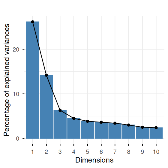
fviz_pca_ind(pcaMouse, geom = "point", col.ind = xwt$sampleGroup) +
  ggtitle("") +
  coord_fixed()
We see from tab that the groups are represented rather unequally. To account for this, we reweigh each sample by the inverse of its group size. The function dudi.pca in the ade4 package has a row.w argument into which we can enter the weights. The output of the code is in Figures 7.33 and 7.34.
Preprocessing matrices Multivariate data analyses require “conscious” preprocessing. After consulting all the means, variances and one-dimensional histograms we saw how to rescale and recenter the data.
Projecting onto new variables We saw how we can make projections into lower dimensions (2D planes and 3D are the most frequently used) of high dimensional data without losing too much information. PCA searches for new “more informative” variables that are linear combinations of the original (old) ones.
Matrix decomposition PCA is based on finding decompositions of the matrix \(X\) called SVD. This decomposition provides a lower rank approximation and is equivalent to the eigendecomposition of \(X^tX\). The squares of the singular values are equal to the eigenvalues and to the variances of the new variables. We systematically plotted these values before deciding how many axes are necessary to reproduce the signal in the data.
Two eigenvalues which are quite close can give rise to scores or PC scores which are highly unstable. It is always necessary to look at the screeplot of the eigenvalues and avoid separating the axes corresponding to the these close eigenvalues. This may require using interactive three or four-dimensional projections, which are available in several R packages.
Biplot representations The space of observations is naturally a \(p\)-dimensional space (the \(p\) original variables provide the coordinates). The space of variables is \(n\)-dimensional. Both decompositions we have studied (singular values / eigenvalues and singular vectors / eigenvectors) provide new coordinates for both of these spaces, sometimes we call one the dual of the other. We can plot the projection of both the observations and the variables onto the same eigenvectors. This provides a biplot that can be useful for interpreting the PCA output.
Projecting other group variables Interpretation of PCA can also be facilitated by redundant or contiguous data about the observations.
The best way to deepen your understanding of singular value decomposition is to read Chapter 7 of Strang (2009). The whole book sets the foundations for the linear algebra necessary to understanding the meaning of the rank of matrix and the duality between row spaces and column spaces (Holmes 2006).
Complete textbooks have been written on the subject of PCA and related methods. Mardia et al. (1979) is a standard text that covers all multivariate methods in a classical way, with linear algebra and matrices. By making the parametric assumptions that the data come from multivariate normal distributions, Mardia et al. (1979) also provide inferential tests for the number of components and limiting properties for principal components. Jolliffe (2002) is a book-long treatment of everything to do with PCA with extensive examples.
We can incorporate supplementary information into weights for the observations and the variables. This was introduced in the 1970’s by French data scientists, see Holmes (2006) for a review and Chapter 9 for further examples.
Improvements to the interpretation and stability of PCA can be obtained by adding a penalty that minimizes the number of nonzero coefficients that appear in the linear combinations. Zou et al. (2006) and Witten et al. (2009) have developed sparse versions of principal component analysis, and their packages elasticnet and PMA provide implementations in R.
library("MASS")
mu1 = 1
mu2 = 2
s1 = 2.5
s2 = 0.8
rho = 0.9
sigma = matrix(c(s1^2, s1 * s2 * rho, s1 * s2 * rho, s2^2), 2)
sim2d = data.frame(mvrnorm(50, mu = c(mu1, mu2), Sigma = sigma))
svd(scale(sim2d))$d
[1] 9.70 1.99svd(scale(sim2d))$v[, 1][1] -0.707 -0.707prcomp to perform a PCA and the scores provide the desired rotation.respc = princomp(sim2d)
dfpc = data.frame(pc1 = respc$scores[, 1], pc2 = respc$scores[, 2])
ggplot(data.frame(sim2d), aes(x = X1, y = X2)) + geom_point()
ggplot(dfpc, aes(x = pc1, y = pc2)) + geom_point() + coord_fixed(2)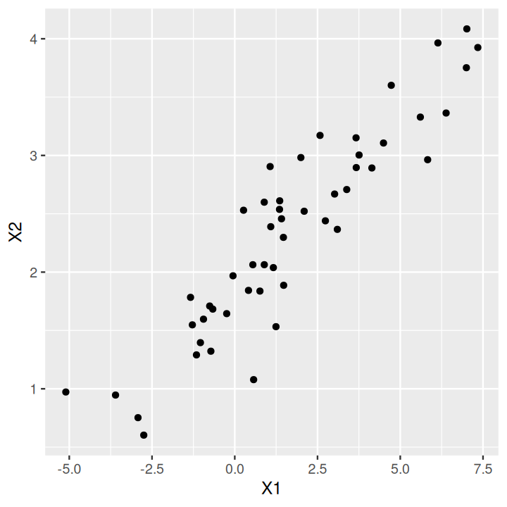
Page built at 21:15 on 2026-07-15 using R version 4.6.0 (2026-04-24)