In a supervised learning setting, we have a yardstick or plumbline to judge how well we are doing: the response itself.
A frequent question in biological and biomedical applications is whether a property of interest (say, disease type, cell type, the prognosis of a patient) can be “predicted”, given one or more other properties, called the predictors. Often we are motivated by a situation in which the property to be predicted is unknown (it lies in the future, or is hard to measure), while the predictors are known. The crucial point is that we learn the prediction rule from a set of training data in which the property of interest is also known. Once we have the rule, we can either apply it to new data, and make actual predictions of unknown outcomes; or we can dissect the rule with the aim of better understanding the underlying biology.
Compared to unsupervised learning and what we have seen in Chapters 5, 7 and 9, where we do not know what we are looking for or how to decide whether our result is “right”, we are on much more solid ground with supervised learning: the objective is clearly stated, and there are straightforward criteria to measure how well we are doing.
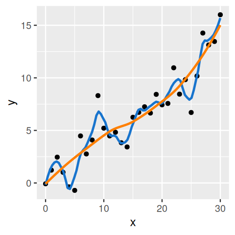
The central issues in supervised learning1 are overfitting and generalizability: did we just learn the training data “by heart” by constructing a rule that has 100% accuracy on the training data, but would perform poorly on any new data? Or did our rule indeed pick up some of the pertinent patterns in the system being studied, which will also apply to yet unseen new data? (Figure 12.1)
1 Sometimes the term statistical learning is used, more or less exchangeably.
Figure 12.1: An example for overfitting: two regression lines are fit to data in the \((x, y)\)-plane (black points). We can think of such a line as a rule that predicts the \(y\)-value, given an \(x\)-value. Both lines are smooth, but the fits differ in what is called their bandwidth, which intuitively can be interpreted their stiffness. The blue line seems overly keen to follow minor wiggles in the data, while the orange line captures the general trend but is less detailed. The effective number of parameters needed to describe the blue line is much higher than for the orange line. Also, if we were to obtain additional data, it is likely that the blue line would do a worse job than the orange line in modeling the new data. We’ll formalize these concepts –training error and test set error– later in this chapter. Although exemplified here with line fitting, the concept applies more generally to prediction models.
12.1 Goals for this chapter
In this chapter we will:
See exemplary applications that motivate the use of supervised learning methods.
Learn what discriminant analysis does.
Define measures of performance.
Encounter the curse of dimensionality and see what overfitting is.
Find out about regularization – in particular, penalization – and understand the concepts of generalizability and model complexity.
See how to use cross-validation to tune parameters of algorithms.
Discuss method hacking.
12.2 What are the data?
The basic data structure for both supervised and unsupervised learning is (at least conceptually) a dataframe, where each row corresponds to an object and the columns are different features (usually numerical values) of the objects2. While in unsupervised learning we aim to find (dis)similarity relationships between the objects based on their feature values (e.g., by clustering or ordination), in supervised learning we aim to find a mathematical function (or a computational algorithm) that predicts the value of one of the features from the other features. Many implementations require that there are no missing values, whereas other methods can be made to work with some amount of missing data.
2 This is a simplified description. Machine learning is a huge field, and lots of generalizations of this simple conceptual picture have been made. Already the construction of relevant features is an art by itself — we have seen examples with images of cells in Chapter 11, and more generally there are lots of possibilities to extract features from images, sounds, movies, free text, \(...\) Moreover, there is a variant of machine learning methods called kernel methods that do not need features at all; instead, kernel methods use distances or measures of similarity between objects. It may be easier, for instance, to define a measure of similarity between two natural language text objects than to find relevant numerical features to represent them. Kernel methods are beyond the scope of this book.
The feature that we select over all the others with the aim of predicting is called the objective or the response. Sometimes the choice is natural, but sometimes it is also instructive to reverse the roles, especially if we are interested in dissecting the prediction function for the purpose of biological understanding, or in disentangling correlations from causation.
The framework for supervised learning covers both continuous and categorical response variables. In the continuous case we also call it regression, in the categorical case, classification. It turns out that this distinction is not a detail, as it has quite far-reaching consequences for the choice of loss function (Section 12.5) and thus the choice of algorithm (Friedman 1997).
The first question to consider in any supervised learning task is how the number of objects compares to the number of predictors. The more objects, the better, and much of the hard work in supervised learning has to do with overcoming the limitations of having a finite (and typically, too small) training set.
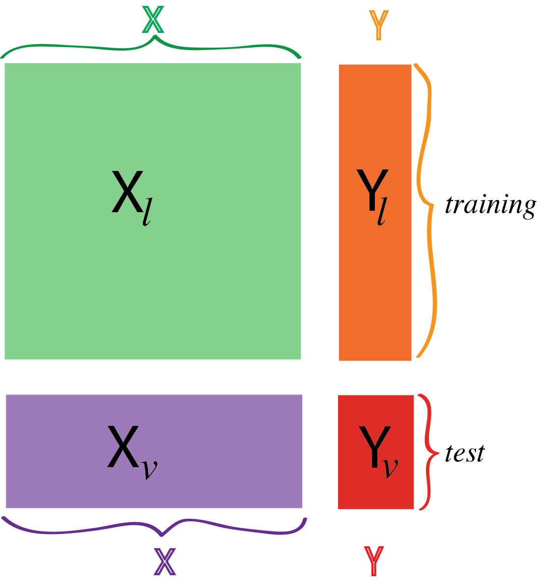
Figure 12.2: In supervised learning, we assign two different roles to our variables. We have labeled the explanatory variables \(X\) and the response variable(s) \(Y\). There are also two different sets of observations: the training set \(X_\ell\) and \(Y_\ell\) and the test set \(X_v\) and \(Y_v\). (The subscripts refer to alternative names for the two sets: “learning” and “validation”.)
Task
Give examples where we have encountered instances of supervised learning with a categorical response in this book.
12.2.1 Motivating examples
Predicting diabetes type
The diabetes dataset (Reaven and Miller 1979) presents three different groups of diabetes patients and five clinical variables measured on them.
data("diabetes", package ="rrcov")head(diabetes)
    rw fpg glucose insulin sspg  group
1 0.81  80     356     124   55 normal
2 0.95  97     289     117   76 normal
3 0.94 105     319     143  105 normal
4 1.04  90     356     199  108 normal
5 1.00  90     323     240  143 normal
6 0.76  86     381     157  165 normal
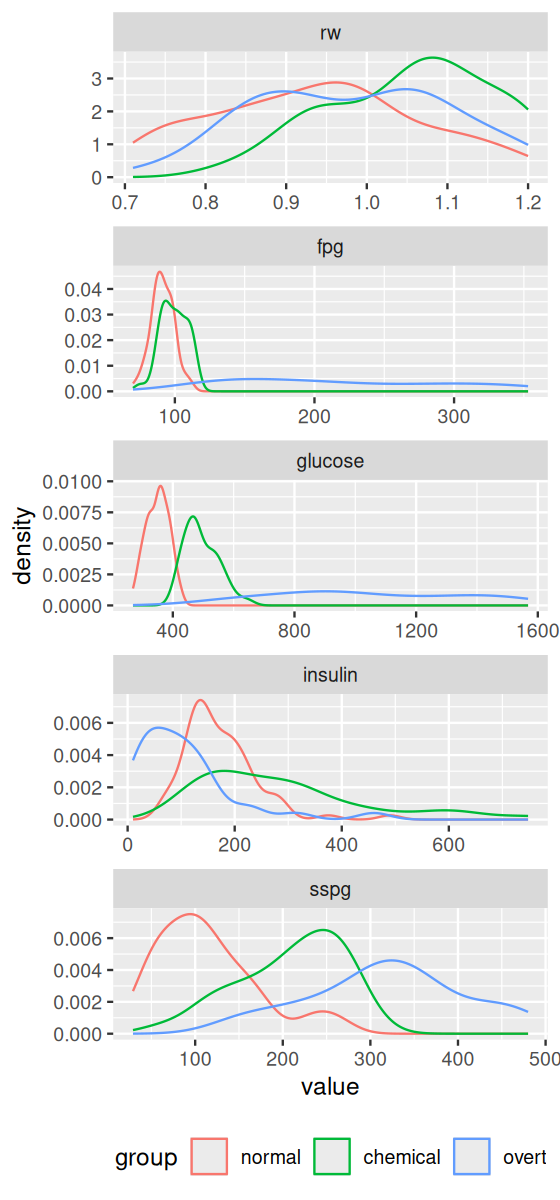
The univariate distributions (more precisely, some density estimates of them) are shown in Figure 12.3.
Figure 12.3: We see already from the one-dimensional distributions that some of the individual variables could potentially predict which group a patient is more likely to belong to. Our goal is to combine variables to improve over such one-dimensional prediction models.
The variables are explained in the manual page of the dataset, and in the paper (Reaven and Miller 1979):
rw: relative weight
fpg: fasting plasma glucose
glucose: area under the plasma glucose curve for the three hour oral glucose tolerance test (OGTT)
insulin: area under the plasma insulin curve for the OGTT
sspg: steady state plasma glucose response
group: normal, chemical diabetes and overt diabetes
Predicting cellular phenotypes
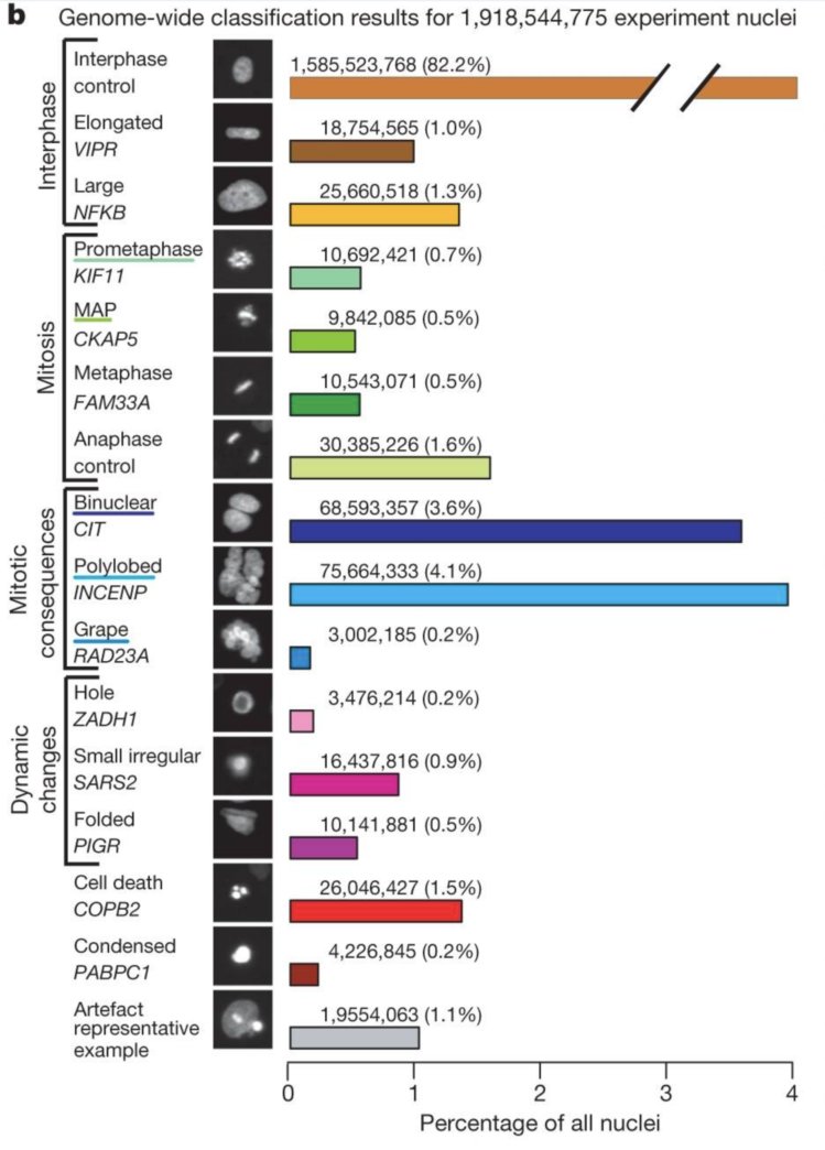
Neumann et al. (2010) observed human cancer cells using live-cell imaging. The cells were genetically engineered so that their histones were tagged with a green fluorescent protein (GFP). A genome-wide RNAi library was applied to the cells, and for each siRNA perturbation, movies of a few hundred cells were recorded for about two days, to see what effect the depletion of each gene had on cell cycle, nuclear morphology and cell proliferation. Their paper reports the use of an automated image classification algorithm that quantified the visual appearance of each cell’s nucleus and enabled the prediction of normal mitosis states or aberrant nuclei. The algorithm was trained on the data from around 3000 cells that were annotated by a human expert. It was then applied to almost 2 billions images of nuclei (Figure 12.4). Using automated image classification provided scalability (annotating 2 billion images manually would take a long time) and objectivity.
Figure 12.4: The data were images of \(2\times10^9\) nuclei from movies. The images were segmented to identify the nuclei, and numeric features were computed for each nucleus, corresponding to size, shape, brightness and lots of other more or less abstract quantitative summaries of the joint distribution of pixel intensities. From the features, the cells were classified into 16 different nuclei morphology classes, represented by the rows of the barplot. Representative images for each class are shown in black and white in the center column. The class frequencies, which are very unbalanced, are shown by the lengths of the bars.
Predicting embryonic cell states
We will revisit the mouse embryo data (Ohnishi et al. 2014), which we have already seen in Chapters 3, 5 and 7. We’ll try to predict cell state and genotype from the gene expression measurements in Sections 12.3.2 and 12.6.3.
12.3 Linear discrimination
We start with one of the simplest possible discrimination problems3: we have objects described by two continuous features (so the objects can be thought of as points in the 2D plane) and falling into three groups. Our aim is to define class boundaries, which are lines in the 2D space.
3 Arguably the simplest possible problem is a single continuous feature, two classes, and the task of finding a single threshold to discriminate between the two groups – as in Figure 6.2.
12.3.1 Diabetes data
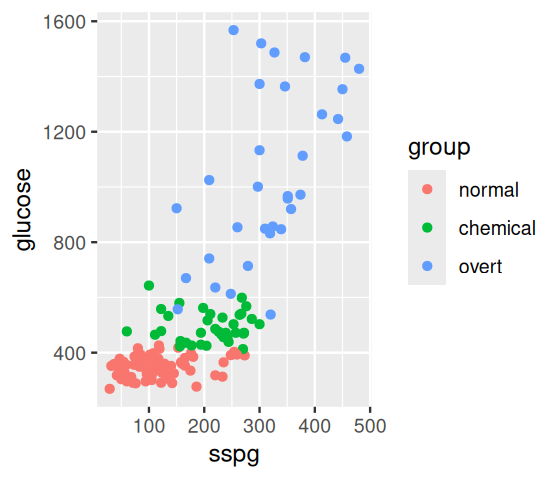
Let’s see whether we can predict the group from the sspg and glucose variables in the diabetes data. It’s always a good idea to first visualise the data (Figure 12.5).
ggdb =ggplot(mapping =aes(x = sspg, y = glucose)) +geom_point(aes(colour = group), data = diabetes)ggdb
Figure 12.5: Scatterplot of two of the variables in the diabetes data. Each point is a sample, and the color indicates the diabetes type as encoded in the group variable.
We’ll start with a method called linear discriminant analysis (LDA). This method is a foundation stone of classification, many of the more complicated (and sometimes more powerful) algorithms are really just generalizations of LDA.
library("MASS")diabetes_lda =lda(group ~ sspg + glucose, data = diabetes)diabetes_lda
Call:
lda(group ~ sspg + glucose, data = diabetes)

Prior probabilities of groups:
   normal  chemical     overt
0.5241379 0.2482759 0.2275862

Group means:
             sspg   glucose
normal   114.0000  349.9737
chemical 208.9722  493.9444
overt    318.8788 1043.7576

Coefficients of linear discriminants:
                LD1         LD2
sspg    0.005036943 -0.01539281
glucose 0.005461400  0.00449050

Proportion of trace:
   LD1    LD2
0.9683 0.0317
ghat       normal chemical overt
  normal       69       12     1
  chemical      7       24     6
  overt         0        0    26
mean(ghat != diabetes$group)
[1] 0.1793103
Question 12.1
What do the different parts of the above output mean?
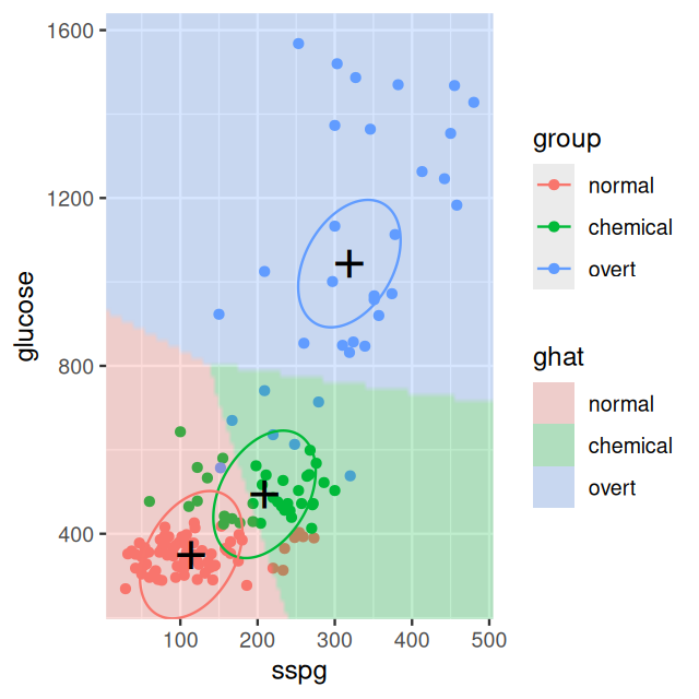
Now, let’s visualise the LDA result. We are going to plot the prediction regions for each of the three groups. We do this by creating a grid of points and using our prediction rule on each of them. We’ll then also dig a bit deeper into the mechanics of LDA and plot the class centers (diabetes_lda$means) and ellipses that correspond to the fitted covariance matrix (diabetes_lda$scaling). Assembling this visualization requires us to write a bit of code.
Compute the ellipse. We start from a unit circle (approximated by a polygon with 360 sides) and apply the corresponding affine transformation from the LDA output.
Figure 12.6: As Figure 12.5, with the classification regions from the LDA model shown. The three ellipses represent the class centers and the covariance matrix of the LDA model; note that there is only one covariance matrix, which is the same for all three classes. Therefore also the sizes and orientations of the ellipses are the same for the three classes, only their centers differ. They represent contours of equal class membership probability.
Question 12.2
Why is the boundary between the prediction regions for chemical and overt not perpendicular to the line between the group centers?
Solution
The boundaries would be perpendicular if the ellipses were circles. In general, a boundary is tangential to the contours of equal class probabilities, and due the elliptic shape of the contours, a boundary is in general not perpendicular to the line between centers.
Question 12.3
How confident would you be about the predictions in those areas of the 2D plane that are far from all of the cluster centers?
Solution
Predictions that are far from any cluster center should be assessed critically, as this amounts to an extrapolation into regions where the LDA model may not be very good and/or there may be no training data nearby to support the prediction. We could use the distance to the nearest center as a measure of confidence in the prediction for any particular point; although we will see that resampling and cross-validation based methods offer more generic and usually more reliable measures.
Question 12.4
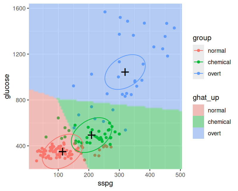
Why is the boundary between the prediction regions for normal and chemical not half-way between the centers, but shifted in favor of normal? Hint: have a look at the prior argument of lda. Try again with uniform prior.
Solution
The result of the following code chunk is shown in Figure 12.7. The suffix _up is short for “uniform prior”.
Figure 12.7: As Figure 12.6, but with uniform class priors.
The stopifnot line confirms that the class centers are the same, as they are independent of the prior. The joint covariance is not.
Question 12.5
Figures 12.6 and 12.7 show both the fitted LDA model, through the ellipses, and the prediction regions, through the area coloring. What part of this visualization is generic for all sorts of classification methods, what part is method-specific?
Solution
The prediction regions can be shown for any classification method, including a “black box” method. The cluster centers and ellipses in Figures 12.6 and 12.7 are method-specific.
Question 12.6
What is the difference in the prediction accuracy if we use all 5 variables instead of just glucose and sspg?
ghat5      normal chemical overt
  normal       73        5     1
  chemical      3       31     5
  overt         0        0    27
mean(ghat5 != diabetes$group)
[1] 0.09655172
Question 12.7
Instead of approximating the prediction regions by classification from a grid of points, compute the separating lines explicitly from the linear determinant coefficients.
12.3.2 Predicting embryonic cell state from gene expression
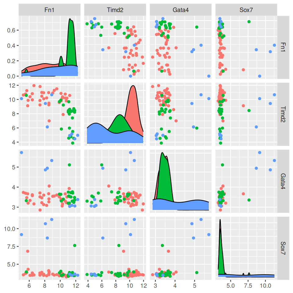
Assume that we already know that the four genes FN1, TIMD2, GATA4 and SOX7 are relevant to the classification task4. We want to build a classifier that predicts the developmental time (embryonic days: E3.25, E3.5, E4.5). We load the data and select four corresponding probes.
4 Later in this chapter we will see methods that can drop this assumption and screen all available features.
Figure 12.8: Expression values of the discriminating genes, with the prediction target Embryonic.day shown by color.
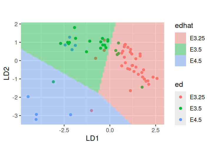
We can now call lda on these data. The linear combinations LD1 and LD2 that serve as discriminating variables are given in the slot ed_lda$scaling of the output from lda.
For the visualization of the learned model in Figure 12.9, we need to build the prediction regions and their boundaries by expanding the grid in the space of the two new coordinates LD1 and LD2.
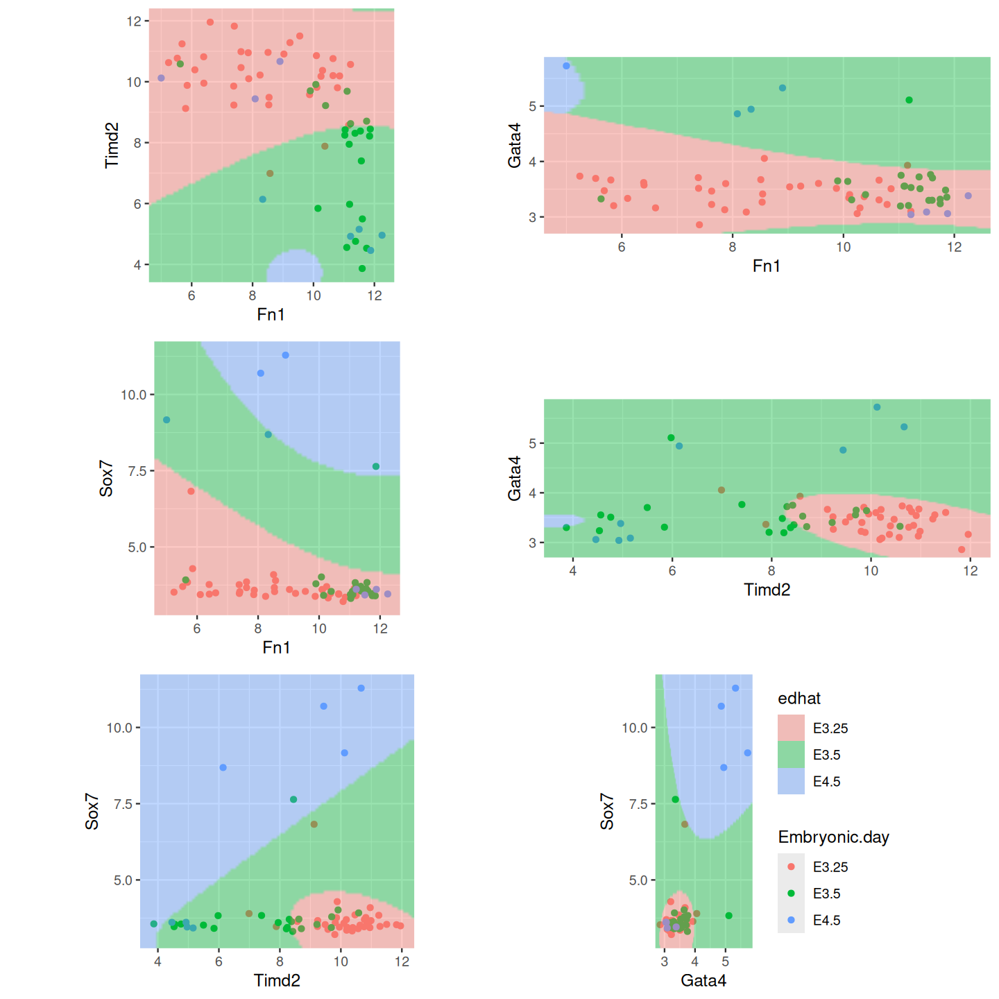
Figure 12.10: QDA for the mouse cell data. Shown are all pairwise plots of the four features. In each plot, the other two features are set to the median.
Question 12.9
What happens if you call lda or qda with a lot more genes, say the first 1000, in the Hiiragi dataset?
Error in `qda.default()`:
! some group is too small for 'qda'
The lda function manages to fit a model, but complains (with the warning) about the fact that there are more variables than replicates, which means that the variables are not linearly independent, and thus are redundant of each other. The qda function aborts with an error, since the QDA model with so many parameters cannot be fitted from the available data (at least, without making further assumptions, such as some sort of regularization, which it is not equipped for).
12.4 Machine learning vs rote learning
Computers are really good at memorizing facts. In the worst case, a machine learning algorithm is a roundabout way of doing this5. The central goal in statistical learning, however, is generalizability. We want an algorithm that is able to generalize, i.e., interpolate and extrapolate from given data to make good predictions about future data.
5 The not-so roundabout way is database technologies.
Let’s look at the following example. We generate random data (rnorm) for n objects, with different numbers of features (given by p). We train a LDA on these data and compute the misclassification rate, i.e., the fraction of times the prediction is wrong (pred != resp).
p =2:21n =20mcl =lapply(p, function(pp) {replicate(100, { xmat =matrix(rnorm(n * pp), nrow = n) resp =sample(c("apple", "orange"), n, replace =TRUE) fit =lda(xmat, resp) pred =predict(fit)$classmean(pred != resp) }) |>mean() |> (\(x) tibble(mcl = x, p = pp))()}) |>bind_rows()
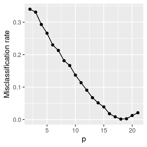
Figure 12.11: Misclassification rate of LDA applied to random data. While the number of observations n is held constant (at 20), we are increasing the number of features p starting from 2 up to 21. The misclassification rate becomes almost zero as p approaches 20. The LDA model becomes so elaborate and over-parameterized that it manages to learn the random labels “by heart”. (As p becomes even larger, the “performance” degrades again somewhat, apparently due to numerical properties of the lda implementation used here.)
Question 12.10
What is the purpose of the replicate loop in the above code? What happens if you omit it (or replace the 100 by 1)?
Solution
For each single replicate, the curve is a noisier version of Figure 12.11. Averaging the measured misclassifications rate over 100 replicates makes the estimate more stable. We can do this since we are working with simulated data.
Figure 12.11 seems to imply that we can perfectly predict random labels from random data, if we only fit a complex enough model, i.e., one with many parameters. How can we overcome such an absurd conclusion? The problem with the above code is that the model performance is evaluated on the same data on which it was trained. This generally leads to positive bias, as you see in this crass example. How can we overcome this problem? The key idea is to assess model performance on different data than those on which the model was trained.
12.4.1 Cross-validation
A naive approach might be to split the data in two halves, and use the first half for learning (“training”) and the second half for assessment (“testing”). It turns out that this is needlessly variable and needlessly inefficient. It is needlessly variable, since by splitting the data only once, our results can be quite affected by how the split happens to fall. It seems better to do the splitting many times, and average. This will give us more stable results. It is needlessly inefficient, since the performance of machine learning algorithms depends on the number of observations, and the performance measured on half the data is likely6 to be worse than what it is with all the data. For this reason, it is better to use unequal sizes of training and test data. In the extreme case, we’ll use as much as \(n-1\) observations for training, and the remaining one for testing. After we’ve done this likewise for all observations, we can average our performance metric. This is called leave-one-out cross-validation.
6 Unless we have such an excess of data that it doesn’t matter.
See Chapter Model Assessment and Selection in the book by Hastie et al. (2008) for further discussion on these trade-offs.
An alternative is \(k\)-fold cross-validation, where the observations are repeatedly split into a training set of size of around \(n(k-1)/k\) and a test set of size of around \(n/k\). Both alternatives have pros and contras, and there is not a universally best choice. An advantage of leave-one-out is that the amount of data used for training is close to the maximally available data; this is especially important if the sample size is limiting and “every little matters” for the algorithm. A drawback of leave-one-out is that the training sets are all very similar, so they may not model sufficiently well the kind of sampling changes to be expected if a new dataset came along. For large \(n\), leave-one-out cross-validation can be needlessly time-consuming.
ggplot(mcl, aes(x = p, y = value, col = variable)) +geom_line() +geom_point() +ylab("Misclassification rate")
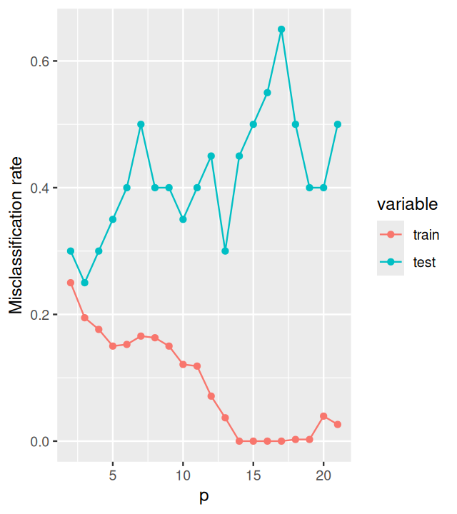
Figure 12.12: Cross-validation: the misclassification rate of LDA applied to random data, when evaluated on test data that were not used for learning, hovers around 0.5 independent of p. The misclassification rate on the training data is also shown. It behaves similar to what we already saw in Figure 12.11.
Why are the curves in Figure 12.12 more variable (“wiggly”) than in Figure 12.11? How can you overcome this?
Solution
Only one dataset (xmat, resp) was used to calculate Figure 12.12, whereas for Figure 12.11, we had the data generated within a replicate loop. You could similarly extend the above code to average the misclassification rate curves over many replicate simulated datasets.
12.4.2 The curse of dimensionality
In Section 12.4.1 we have seen overfitting and cross-validation on random data, but how does it look if there is in fact a relevant class separation?
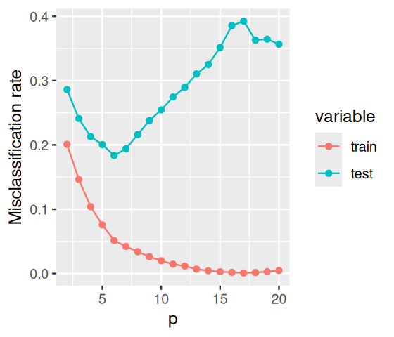
mcl =group_by(mcl, p, variable) |>summarise(value =mean(value))ggplot(mcl, aes(x = p, y = value, col = variable)) +geom_line() +geom_point() +ylab("Misclassification rate")
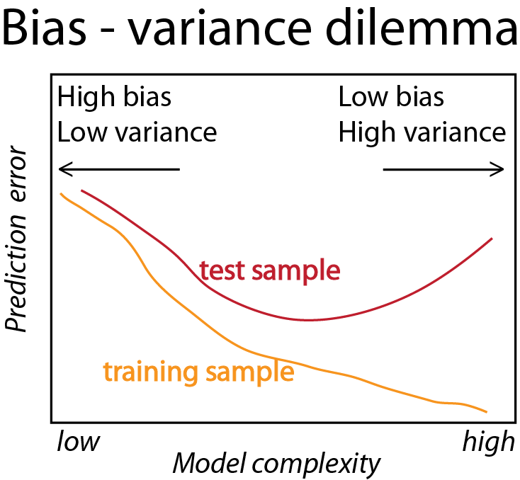
Figure 12.13: As we increase the number of features included in the model, the misclassification rate initially improves; as we start including more and more irrelevant features, it increases again, as we are fitting noise.
Figure 12.14: Idealized version of Figure 12.13, from Hastie et al. (2008). A recurrent goal in machine learning is finding the sweet spot in the variance <- bias trade-off.
The result is shown in Figure 12.13. The group centers are the vectors (in \(\mathbb{R}^{20}\)) given by the coordinates \((1, 1, 1, 1, 1, 1, 0, 0, 0, ...)\) (apples) and \((2, 2, 2, 2, 2, 2, 0, 0, 0, ...)\) (oranges), and the optimal decision boundary is the hyperplane orthogonal to the line between them. For \(p\) smaller than \(6\), the decision rule cannot reach this hyperplane – it is biased. As a result, the misclassification rate is suboptimal, and it decreases with \(p\). But what happens for \(p\) larger than \(6\)? The algorithm is, in principle, able to model the optimal hyperplane, and it should not be distracted by the additional features. The problem is that it is. The more additional features enter the dataset, the higher the probability that one or more of them happen to fall in a way that they look like good, discriminating features in the training data – only to mislead the classifier and degrade its performance in the test data. Shortly we’ll see how to use penalization to (try to) control this problem.
The term curse of dimensionality was coined by Bellman (1961). It refers to the fact that high-dimensional spaces are very hard, if not impossible, to sample thoroughly: for instance, to cover a 2-dimensional square of side length 1 with grid points that are 0.1 apart, we need \(10^2=100\) points. In 100 dimensions, we need \(10^{100}\) – which is more than the number of protons in the universe. In genomics, we often aim to fit models to data with thousands of features. Also our intuitions about distances between points or about the relationship between a volume and its surface break down in a high-dimensional settings. We’ll explore some of the weirdnesses of high-dimensional spaces in the next few questions.
Question 12.12
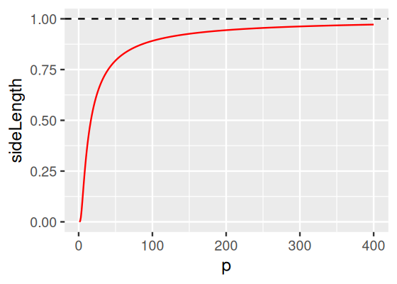
Assume you have a dataset with 1 000 000 data points in \(p\) dimensions. The data are uniformly distributed in the unit hybercube (i.e., all features lie in the interval \([0,1]\)). What’s the side length of a hybercube that can be expected to contain just 10 of the points, as a function of \(p\)?
Figure 12.15: Side length of a \(p\)-dimensional hybercube expected to contain 10 points out of 1 million uniformly distributed ones, as a function of the \(p\). While for \(p=1\), this length is conveniently small, namely \(10/10^6=10^{-5}\), for larger \(p\) it approaches 1, i.,e., becomes the same as the range of each the features. This means that a “local neighborhood” of 10 points encompasses almost the same data range as the whole dataset.
Next, let’s look at the relation between inner regions of the feature space versus its boundary regions. Generally speaking, prediction at the boundaries of feature space is more difficult than in its interior, as it tends to involve extrapolation, rather than interpolation. In the next question you’ll see how this difficulty explodes with feature space dimension.
Question 12.13
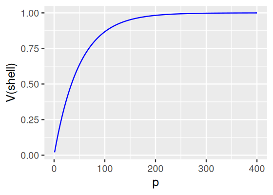
What fraction of a unit cube’s total volume is closer than 0.01 to any of its surfaces, as a function of the dimension?
Figure 12.16: Fraction of a unit cube’s total volume that is in its “shell” (here operationalised as those points that are closer than 0.01 to its surface) as a function of the dimension \(p\).
Question 12.14
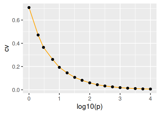
What is the coefficient of variation (ratio of standard deviation over average) of the distance between two randomly picked points in the unit hypercube, as a function of the dimension?
Solution
We solve this one by simulation. We generate n pairs of random points in the hypercube (x1, x2) and compute their Euclidean distances. See Figure 12.17. This result can also be predicted from the central limit theorem.
n =1000df =tibble(p =round(10^seq(0, 4, by =0.25)),cv =vapply(p, function(k) { x1 =matrix(runif(k * n), nrow = n) x2 =matrix(runif(k * n), nrow = n) d =sqrt(rowSums((x1 - x2)^2))sd(d) /mean(d) }, FUN.VALUE =numeric(1)))ggplot(df, aes(x =log10(p), y = cv)) +geom_line(col ="orange") +geom_point()
Figure 12.17: Coefficient of variation (CV) of the distance between randomly picked points in the unit hypercube, as a function of the dimension. As the dimension increases, everybody is equally far away from everyone else: there is almost no variation in the distances any more.
12.5 Objective functions
We’ve already seen the misclassification rate (MCR) used to assess our classification performance in Figures 12.11–12.13. Its population version is defined as
This is not the only choice we could make. Perhaps we care more about the misclassification of apples as oranges than vice versa, and we can reflect this by introducing weights that depend on the type of error made into the sum of Equation 12.2 (or the integral of Equation 12.1). This can get even more elaborate if we have more than two classes. Often we want to see the whole confusion table, which we can get via
table(truth, response)
An important special case is binary classification with asymmetric costs – think about, say, a medical test. Here, the sensitivity (a.k.a. true positive rate or recall) is related to the misclassification of healthy as ill, and the specificity (or true negative rate) depends on the probability of misclassification of ill as healthy. Often, there is a single parameter (e.g., a threshold) that can be moved up and down, allowing a trade-off between sensitivity and specificity (and thus, equivalently, between the two types of misclassification). In those cases, we usually are not content to know the classifier performance at one single choice of threshold, but at many (or all) of them. This leads to receiver operating characteristic (ROC) or precision-recall curves.
Question 12.15
What are the exact relationships between the per-class misclassification rates and sensitivity and specificity?
Solution
The sensitivity or true positive rate is
\[
\text{TPR} = \frac{\text{TP}}{\text{P}},
\]
where \(\text{TP}\) is the number of true positives and \(\text{P}\) the number of all positives. The specificity or true negative rate is
where \(A\) is the set of observations for which the true class is 1 (\(A=\{i\,|\,y_i=1\}\)) and \(B\) is the set of observations for which the predicted class is 1. The number \(J\) is between 0 and 1, and when \(J\) is large, it indicates high overlap of the two sets. Note that \(J\) does not depend on the number of observations for which both true and predicted class is 0 – so it is particularly suitable for measuring the performance of methods that try to find rare events.
We can also consider probabilistic class predictions, which come in the form \(\hat{P}(Y\,|\,X)\). In this case, a possible risk function would be obtained by looking at distances between the true probability distribution and the estimated probability distributions. For two classes, the finite sample version of the \(\log \text{loss}\) is
The population version is defined analogously, by turning the summation into an integral as in Equations 12.1 and 12.2.
Statisticians call functions like Equations 12.1—12.5 variously (and depending on context and predisposition) risk function, cost function, objective function7.
7 There is even an R package dedicated to evaluation of statistical learners called metrics.
12.6 Variance–bias trade-off
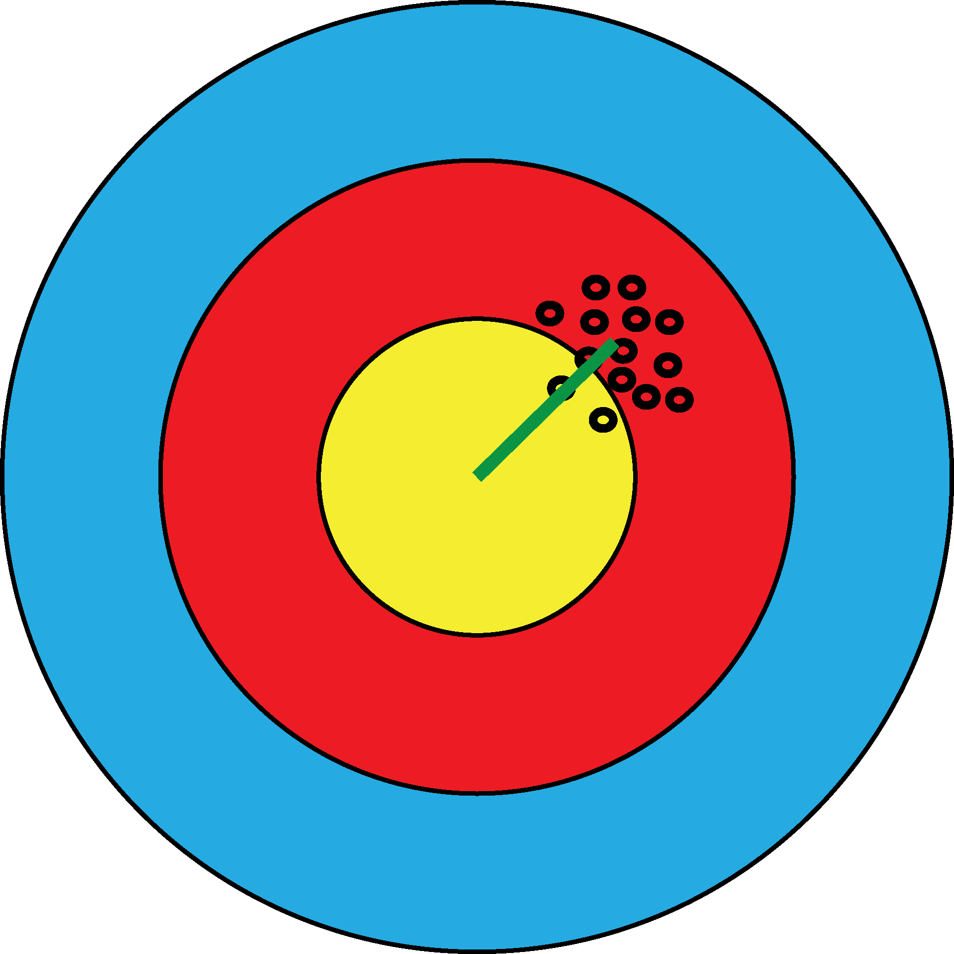
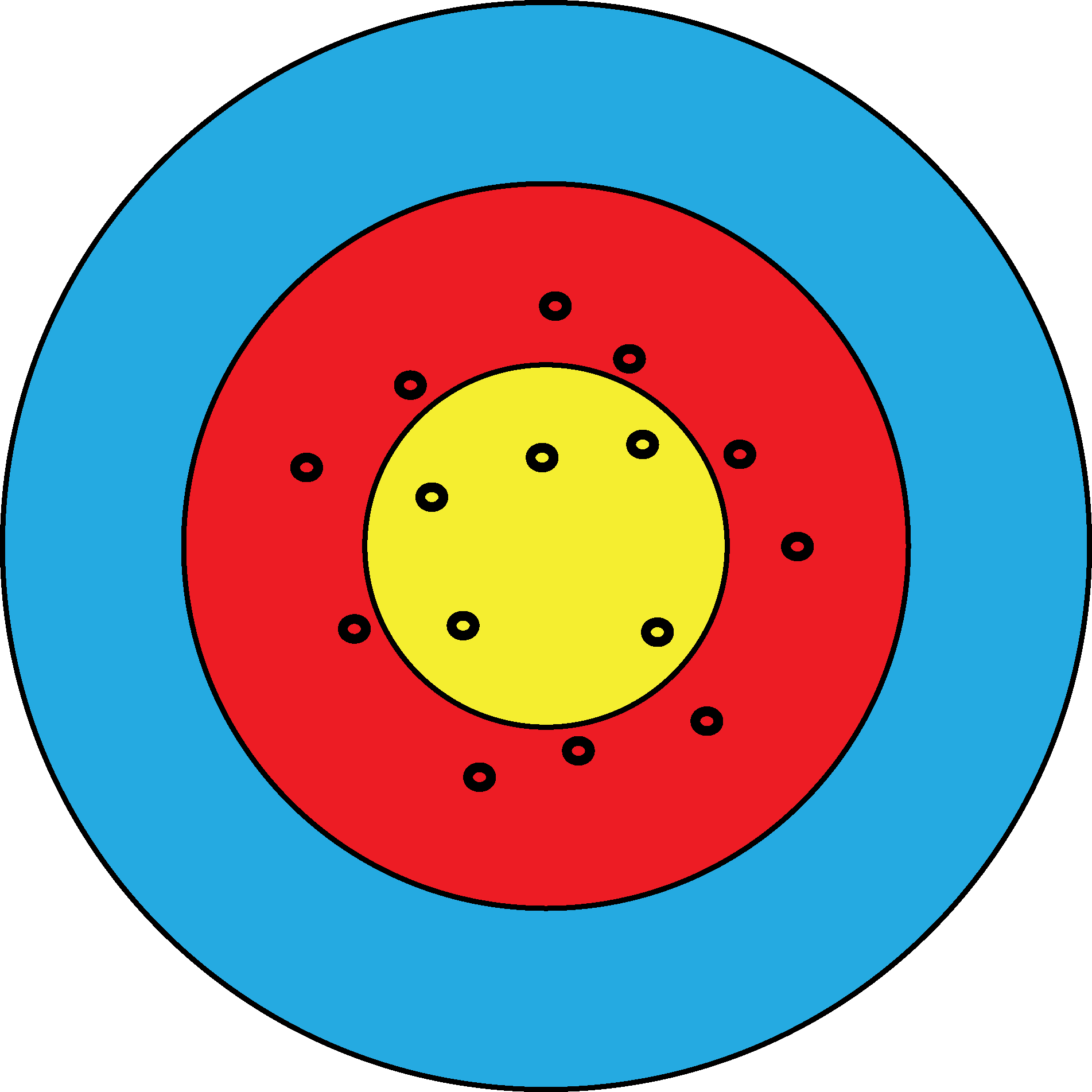
Figure 12.18: In bull’s eye (a), the estimates are systematically off target, but in a quite reproducible manner. The green segment represents the bias. In bull’s eye (b), the estimates are not biased, as they are centered in the right place, however they have high variance. We can distinguish the two scenarios since we see the result from many shots. If we only had one shot and missed the bull’s eye, we could not easily know whether that’s because of bias or variance.
An important fact that helps us understand the tradeoffs when picking a statistical learning model is that the MSE is the sum of two terms, and often the choices we can make are such that one of those terms goes down while the other one goes up. The bias measures how different the average of all the different estimates is from the truth, and variance, how much an individual one might scatter from the average value (Figure 12.18). In applications, we often only get one shot, therefore being reliably almost on target can beat being right on the long term average but really off today. The decomposition
When trying to minimize the MSE, it is important to realize that sometimes we can pay the price of a small bias to greatly reduce variance, and thus overall improve MSE. We already encountered shrinkage estimation in Chapter 8. In classification (i.e., when we have categorical response variables), different objective functions than the MSE are used, and there is usually no such straightforward decomposition as in Equation 12.6. The good news is that we can usually go even much further than in the case of continuous responses with our trading biases for variance. This is because the discreteness of the response absorbs certain biases (Friedman 1997), so that the cost of higher bias is almost zero, while we still get the benefit of better (smaller) variance.
12.6.1 Penalization
In high-dimensional statistics, we are constantly plagued by variance: there is just not enough data to fit all the possible parameters. One of the most fruitful ideas in high-dimensional statistics is penalization: a tool to actively control and exploit the variance-bias tradeoff. Penalization is part of a larger class of regularization methods that are used to ensure stable estimates.
Although generalization of LDA to high-dimensional settings is possible (Clemmensen et al. 2011; Witten and Tibshirani 2011), it turns out that logistic regression is a more general approach8, and therefore we’ll now switch to that, using the glmnet package.
8 It fits into the framework of generalized linear models, which we encountered in Chapter 8.
For multinomial—or, for the special case of two classes, binomial—logistic regression models, the posterior log-odds between \(k\) classes and can be written in the form (see the section on Logistic Regression in the book by Hastie et al. (2008) for a more complete presentation):
where \(i=1,...,k-1\) enumerates the different classes and the \(k\)-th class is chosen as a reference. The data matrix \(x\) has dimensions \(n\times p\), where \(n\) is number of observations and \(p\) the number of features. The \(p\)-dimensional vector \(\beta_i\) determines how the classification odds for class \(i\) versus class \(k\) depend on \(x\). The numbers \(\beta^0_i\) are intercepts and depend, among other things, on the classes’ prior probabilities. Instead of the log odds 12.7 (i.e., ratios of class probabilities), we can also write down an equivalent model for the class probabilities themselves, and the fact that we here used the \(k\)-th class as a reference is an arbitrary choice, as the model estimates are equivariant under this choice (Hastie et al. 2008). The model is fit by maximising the log-likelihood \(\mathcal{l}(\beta, \beta^0; x)\), where \(\beta=(\beta_1,...,\beta_{k-1})\) and analogously for \(\beta^0\).
So far, so good. But as \(p\) gets larger, there is an increasing chance that some of the estimates go wildly off the mark, due to random sampling happenstances in the data (remember Figure 12.1). This is true even if for each individual coordinate of the vector \(\beta_i\), the error distribution is bounded: the probabilty of there being one coordinate that is in the far tails increases the more coordiates there are, i.e., the larger \(p\) is.
A related problem can also occur, not in 12.7, but in other, non-linear models, as the model dimension \(p\) increases while the sample size \(n\) remains the same: the likelihood landscape around its maximum becomes increasingly flat, and the maximum-likelihood estimate of the model parameters becomes more and more variable. Eventually, the maximum is no longer a point, but a submanifold, and the maximum likelihood estimate is unidentifiable. Both of these limitations can be overcome with a modification of the objective: instead of maximising the bare log-likelihood, we maximise a penalized version of it,
where \(\lambda\ge0\) is a real number, and \(\operatorname{pen}\) is a convex function, called the penalty function. Popular choices are \(\operatorname{pen}(\beta)=|\beta|^2\) (ridge regression) and \(\operatorname{pen}(\beta)=|\beta|^1\) (lasso).
Here, \(|\beta|^\nu=\sum_i\beta_i^\nu\) is the \(L_\nu\)-norm of the vector \(\beta\). Variations are possible, for instead we could include in this summation only some but not all of the elements of \(\beta\); or we could scale different elements differently, for instance based on some prior belief of their scale and importance.
In the elastic net, ridge and lasso are hybridized by using the penalty function \(\operatorname{pen}(\beta)=(1-\alpha)|\beta|^1+\alpha|\beta|^2\) with some further parameter \(\alpha\in[0,1]\). The crux is, of course, how to choose the right \(\lambda\), and we will discuss that in the following.
12.6.2 Example: predicting colon cancer from stool microbiome composition
Zeller et al. (2014) studied metagenome sequencing data from fecal samples of 156 humans that included colorectal cancer patients and tumor-free controls. Their aim was to see whether they could identify biomarkers (presence or abundance of certain taxa) that could help with early tumor detection. The data are available from Bioconductor through its ExperimentHub service under the identifier EH361.
Before jumping into model fitting, as always it’s a good idea to do some exploration of the data. First, let’s look at the sample annotations. The following code prints the data from three randomly picked samples. (Only looking at the first ones, say with the R function head, is also an option, but may not be representative of the whole dataset).
pData(zellerNC)[ sample(ncol(zellerNC), 3), ]
                   subjectID age gender bmi country disease tnm_stage
CCIS62794166ST-4-0    FR-780  68   male  23  france  cancer    t3n1m1
CCIS87167916ST-4-0    FR-223  79   male  30  france  cancer    t4n1m1
CCIS17669415ST-4-0    FR-125  72 female  37  france  cancer    t1n0m0
                   ajcc_stage localization     fobt wif-1_gene_methylation_test
CCIS62794166ST-4-0         iv           lc negative                        <NA>
CCIS87167916ST-4-0         iv       rectum positive                    negative
CCIS17669415ST-4-0          i           lc negative                    positive
                   group bodysite ethnicity number_reads
CCIS62794166ST-4-0   crc    stool     white     39333809
CCIS87167916ST-4-0   crc    stool     white     50204707
CCIS17669415ST-4-0   crc    stool     white     69983469
Next, let’s explore the feature names:
We define the helper function formatfn to line wrap these long character strings for the available space here.
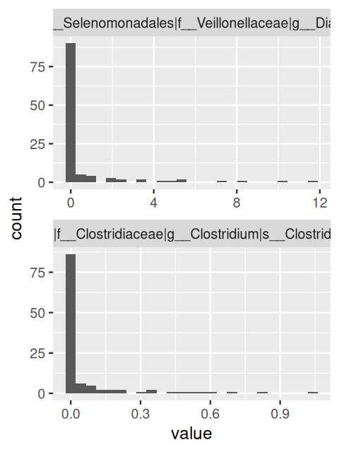
As you can see, the features are a mixture of abundance quantifications at different taxonomic levels, from kingdom over phylum to species. We could select only some of these, but here we continue with all of them. Next, let’s look at the distribution of some of the features. Here, we show an arbitrary choice of two, number 510 and 527; in practice, it is helpful to scroll through many such plots quickly to get an impression (Figure 12.19).
Figure 12.19: Histograms of the distributions for two randomly selected features. The distributions are highly skewed, with many zero values and a thin, long tail of non-zero values.
In the simplest case, we fit model 12.7 as follows.
A remarkable feature of the glmnet function is that it fits 12.7 not only for one choice of \(\lambda\), but for all possible \(\lambda\)s at once. For now, let’s look at the prediction performance for, say, \(\lambda=0.04\). The name of the function parameter is s:
predTrsf =predict(glmfit, newx =t(Biobase::exprs(zellerNC)),type ="class", s =0.04)table(predTrsf, zellerNC$disease)
predTrsf cancer  n
  cancer     51  0
  n           2 61
Not bad – but remember that this is on the training data, without cross-validation. Let’s have a closer look at glmfit. The glmnet package offers a a diagnostic plot that is worth looking at (Figure 12.20).
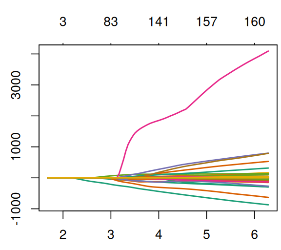
plot(glmfit, col = RColorBrewer::brewer.pal(8, "Dark2"), lwd =sqrt(3), ylab ="")
Figure 12.20: Regularization paths for glmfit.
Question 12.17
What are the \(x\)- and \(y\)-axes in Figure 12.20? What are the different lines?
Solution
Consult the manual page of the function plot.glmnet in the glmnet package.
Let’s get back to the question of how to choose the parameter \(\lambda\). We could try many different choices –and indeed, all possible choices– of \(\lambda\), assess classification performance in each case using cross-validation, and then choose the best \(\lambda\).
You’ll already realize from the description of this strategy that if we optimize \(\lambda\) in this way, the resulting apparent classification performance will likely be exaggerated. We need a truly independent dataset, or at least another, outer cross-validation loop to get a more realistic impression of the generalizability. We will get back to this question at the end of the chapter.
We could do so by writing a loop as we did in the estimate_mcl_loocv function in Section 12.4.1. It turns out that the glmnet package already has built-in functionality for that, with the function cv.glmnet, which we can use instead.
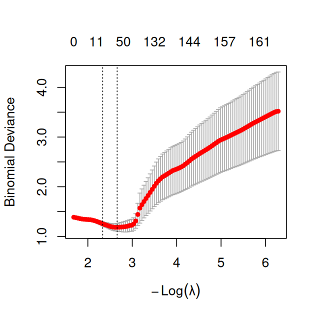
Figure 12.21: Diagnostic plot for cv.glmnet: shown is a measure of cross-validated prediction performance, the deviance, as a function of \(\lambda\). The dashed vertical lines show lambda.min and lambda.1se.
The diagnostic plot is shown in Figure 12.21. We can access the optimal value with
cvglmfit$lambda.min
[1] 0.06998238
As this value results from finding a minimum in an estimated curve, it turns out that it is often too small, i.e., that the implied penalization is too weak. A heuristic recommended by the authors of the glmnet package is to use a somewhat larger value instead, namely the largest value of \(\lambda\) such that the performance measure is within 1 standard error of the minimum.
cvglmfit$lambda.1se
[1] 0.09691764
Question 12.18
How does the confusion table look like for \(\lambda=\;\)lambda.1se?
Solution
s0 = cvglmfit$lambda.1sepredict(glmfit, newx =t(Biobase::exprs(zellerNC)),type ="class", s = s0) |>table(zellerNC$disease)
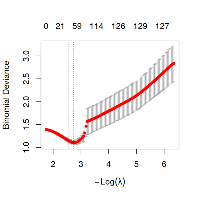
Figure 12.22: like Figure 12.21, but using an \(\text{asinh}\) transformation of the data.
Question 12.21
Would a good classification performance on these data mean that this assay is ready for screening and early cancer detection?
Solution
No. The performance here is measured on a set of samples in which the cases have similar prevalence as the controls. This serves well enough to explore the biology. However, in a real-life application, the cases will be much less frequent. To be practically useful, the assay must have a much higher specificity, i.e., rarely diagnose disease where there is none. To establish specificity, a much larger set of normal samples need to be tested.
12.6.3 Example: classifying mouse cells from their expression profiles
Figures 12.21 and 12.22 are textbook examples of how we expect the dependence of (cross-validated) classification performance versus model complexity (\(\lambda\)) to look. Now let’s get back to the mouse embryo cells data. We’ll try to classify the cells from embryonic day E3.25 with respect to their genotype.
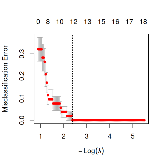
Figure 12.23: Cross-validated misclassification error versus penalty parameter for the mouse cells data.
In Figure 12.23 we see that the misclassification error is (essentially) monotonously increasing with \(\lambda\), and is smallest for \(\lambda\to 0\), i.e., if we apply no penalization at all.
Question 12.22
What is going on with these data?
Solution
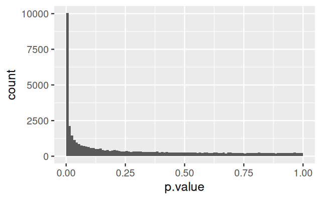
It looks that inclusion of more, and even of all features, does not harm the classification performance. In a way, these data are “too easy”. Let’s do a \(t\)-test for all features:
Figure 12.24: Histogram of p-values for the per-feature \(t\)-tests between genotypes in the E3.25 cells.
The result, shown in Figure 12.24, shows that large number of genes are differentially expressed, and thus informative for the class distinction. We can also compute the pairwise distances between all cells, using all features.
Using all features, the 1 nearest-neighbor classifier is correct in almost all cases, including for the E3.25 wildtype vs FGF4-KO distinction. This means that for these data, there is no apparent benefit in regularization or feature selection. Limitations of using all features might become apparent with truly new data, but that is out of reach for cross-validation.
12.7 A large choice of methods
We have now seen three classification methods: linear discriminant analysis (lda), quadratic discriminant analysis (qda) and logistic regression using elastic net penalization (glmnet). In fact, there are hundreds of different learning algorithms9 available in R and its add-on packages. You can get an overview in the CRAN task view Machine Learning & Statistical Learning. Some examples are:
9 For an introduction to the subject that uses R and provides many examples and exercises, we recommend (James et al. 2013).
Support vector machines: the function svm in the package e1071; ksvm in kernlab
Boosting methods: the functions glmboost and gamboost in package mboost
PenalizedLDA in the package PenalizedLDA, dudi.discr and dist.pcaiv in ade4).
The complexity and heterogeneity of choices of learning strategies, tuning parameters and evaluation criteria in each of these packages can be confusing. You will already have noted differences in the interfaces of the lda, qda and glmnet functions, i.e., in how they expect their input data to presented and what they return. There is even greater diversity across all the other packages and functions. At the same time, there are common tasks such as cross-validation, parameter tuning and performance assessment that are more or less the same no matter what specific method is used. As you have seen, e.g., in our estimate_mcl_loocv function, the looping and data shuffling involved led to rather verbose code.
So what to do if you want to try out and explore different learning algorithms? Fortunately, there are several projects that provide unified interfaces to the large number of different machine learning interfaces in R, and also try to provide “best practice” implementations of the common tasks such as parameter tuning and performance assessment. The two most well-known ones are the packages caret and mlr. Here were have a look at caret. You can get a list of supported methods through its getModelInfo function. There are quite a few, here we just show the first 8.
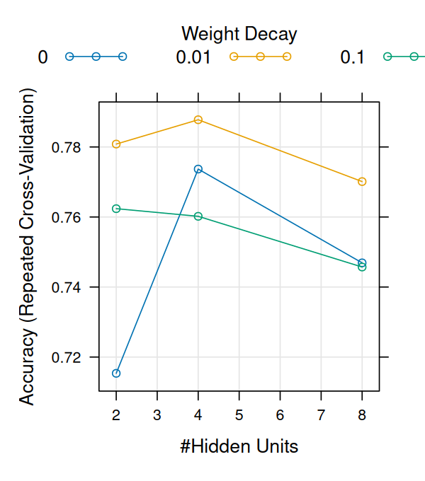
We will check out a neural network method, the nnet function from the eponymous package. The parameter slot informs us on the the available tuning parameters10.
10 They are described in the manual of the nnet function.
That’s quite a mouthful, but the nice thing is that this syntax is standardized and applies across many different methods. All you need to do specify the name of the method and the grid of tuning parameters that should be explored via the tuneGrid argument.
Now we can have a look at the output (Figure 12.25).
nnfit
Neural Network

66 samples
 4 predictor
 3 classes: 'E3.25', 'E3.5', 'E4.5'

No pre-processing
Resampling: Cross-Validated (10 fold, repeated 3 times)
Summary of sample sizes: 59, 59, 60, 60, 60, 60, ...
Resampling results across tuning parameters:

  size  decay  Accuracy   Kappa
  2     0.00   0.7153571  0.4763093
  2     0.01   0.7808333  0.6185837
  2     0.10   0.7623810  0.5804533
  4     0.00   0.7736905  0.6059126
  4     0.01   0.7877778  0.6282527
  4     0.10   0.7601984  0.5719479
  8     0.00   0.7469048  0.5700943
  8     0.01   0.7701190  0.5954734
  8     0.10   0.7457143  0.5471589

Accuracy was used to select the optimal model using the largest value.
The final values used for the model were size = 4 and decay = 0.01.
Figure 12.25: Parameter tuning of the neural net by cross-validation.
Question 12.23
Will the accuracy that we obtained above for the optimal tuning parameters generalize to a new dataset? What could you do to address that?
Solution
No, it is likely to be too optimistic, as we have picked the optimum. To get a somewhat more realistic estimate of prediction performance when generalized, we could formalize (into computer code) all our data preprocessing choices and the above parameter tuning procedure, and embed this in another, outer cross-validation loop (Ambroise and McLachlan 2002). However, this is likely still not enough, as we discuss in the next section.
12.7.1 Method hacking
In Chapter 6 we encountered p-value hacking. A similar phenomenon exists in statistical learning: given a dataset, we explore various different methods of preprocessing (such as normalization, outlier detection, transformation, feature selection), try out different machine learning algorithms and tune their parameters until we are content with the result. The measured accuracy is likely to be too optimistic, i.e., will not generalize to a new dataset. Embedding as many of our methodical choices into a computational formalism and having an outer cross-validation loop (not to be confused with the inner loop that does the parameter tuning) will ameliorate the problem. But is unlikely to address it completely, since not all our choices can be formalized.
The gold standard remains validation on truly unseen data. In addition, it is never a bad thing if the classifier is not a black box but can be interpreted in terms of domain knowledge. Finally, report not just summary statistics, such as misclassification rates, but lay open the complete computational workflow, so that anyone (including your future self) can convince themselves of the robustness of the result or of the influence of the preprocessing, model selection and tuning choices (Holmes 2018).
12.8 Summary of this chapter
We have seen examples of machine learning applications; we have focused on predicting categorical variables (like diabetes type or cell class). Predicting continuous outcomes is also part of machine learning, although we have not considered it here. There are many parallels and overlaps between machine learning and statistical regression (which we studied in Chapter 8). One can consider them two different names for pretty much the same activity, although each has its own flavors: in machine learning, the emphasis is on the prediction of the outcome variables, whereas in regression we often care at least as much about the role of the covariates – which of them have an effect on the outcome, and what is the nature of these effects? In other words, we do not only want predictions, we also want to understand them.
We saw linear and quadratic discriminant analysis, two intuitive methods for partitioning a two-dimensional data plane (or a \(p\)-dimensional space) into regions using either linear or quadratic separation lines (or hypersurfaces). We also saw logistic regression, which takes a slightly different approach but is more amenable to operating in higher dimensions and to regularization.
We encountered the main challenge of machine learning: how to avoid overfitting? We explored why overfitting happens in the context of the so-called curse of dimensionality, and we learned how it may be overcome using regularization.
In other words, machine learning would be easy if we had infinite amounts of data representatively covering the whole space of possible inputs and outputs11. The challenge is to make the best out of a finite amount of training data, and to generalize these to new, unseen inputs. There is a vigorous trade-off between the amount, resolution and coverage of training data and the complexity of the model. Many models have continuous parameters that enable us to “tune” their complexity or the strength of their regularization. Cross-validation can help us with such tuning, although it is not a panacea, and caveats apply, as we saw in Section 12.6.3.
11 It would “just” be a formidable database / data management problem.
12.9 Further reading
An introduction to statistical learning that employs many concrete data examples and uses little mathematical formalism is given by James et al. (2013). An extension, with more mathematical background, is the textbook by Hastie et al. (2008).
Apply a kernel support vector machine, available in the kernlab package, to the zeller microbiome data. What kernel function works well?
Exercise 12.2
Use glmnet for a prediction of a continuous variable, i.e., for regression. Use the prostate cancer data from Chapter 3 of (Hastie et al. 2008). The data are available in the CRAN package ElemStatLearn. Explore the effects of using ridge versus lasso penalty.
Exercise 12.3
Consider smoothing as a regression and model selection problem (remember Figure 12.1). What is the equivalent quantity to the penalization parameter \(\lambda\) in Equation 12.8? How do you choose it?
Scale invariance. Consider a rescaling of one of the features in the (generalized) linear model 12.7. For instance, denote the \(\nu\)-th column of \(x\) by \(x_{\cdot\nu}\), and suppose that \(p\ge2\) and that we rescale \(x_{\cdot\nu} \mapsto s\, x_{\cdot\nu}\) with some number \(s\neq0\). What will happen to the estimate \(\hat{\beta}\) from Equation 12.8 in (a) the unpenalized case (\(\lambda=0\)) and (b) the penalized case (\(\lambda>0\))?
Solution
In the unpenalized case, the estimates will be scaled by \(1/s\), so that the resulting model is, in effect, the same. In the penalized case, the penalty from the \(\nu\)-th component of \(\beta\) will be different. If \(|s|>1\), the amplitude of the feature is increased, smaller \(\beta\)-components are required for it to have the same effect in the prediction, and therefore the feature is more likely to receive a non-zero and/or larger estimate, possibly on the cost of the other features; conversely for \(|s|<1\). Regular linear regression is scale-invariant, whereas penalized regression is scale-dependent. It’s important to remember this when interpreting penalized model fits.
Exercise 12.5
It has been quipped that all classification methods are just refinements of two archetypal ideas: discriminant analysis and \(k\) nearest neighbors. In what sense might that be a useful classification?
Solution
In linear discriminant analysis, we consider our objects as elements of \(\mathbb{R}^p\), and the learning task is to define regions in this space, or boundary hyperplanes between them, which we use to predict the class membership of new objects. This is archetypal for classification by partition. Generalizations of linear discriminant analysis permit more general spaces and more general boundary shapes.
In \(k\) nearest neighbors, no embedding into a coordinate space is needed, but instead we require a distance (or dissimilarity) measure that can be computed between each pair of objects, and the classification decision for a new object depends on its distances to the training objects and their classes. This is archetypal for kernel-based methods.
Page built at 21:16 on 2026-07-15 using R version 4.6.0 (2026-04-24)
Ambroise, Christophe, and Geoffrey J. McLachlan. 2002. “Selection Bias in Gene Extraction on the Basis of Microarray Gene-Expression Data.”PNAS 99 (10): 6562–66.
Bellman, Richard Ernest. 1961. Adaptive Control Processes: A Guided Tour. Princeton University Press.
Friedman, Jerome H. 1997. “On Bias, Variance, 0/1—Loss, and the Curse-of-Dimensionality.”Data Mining and Knowledge Discovery 1: 55–77.
Hastie, Trevor, Robert Tibshirani, and Jerome Friedman. 2008. The Elements of Statistical Learning. \(2^{\text{nd}}\). Springer.
Holmes, Susan. 2018. “Statistical Proof? The Problem of Irreproducibility.”Bulletin of the AMS 55 (1): 31–55.
James, Gareth, Daniela Witten, Trevor Hastie, and Robert Tibshirani. 2013. An Introduction to Statistical Learning. Springer.
Neumann, B., T. Walter, J. K. Heriche, et al. 2010. “Phenotypic profiling of the human genome by time-lapse microscopy reveals cell division genes.”Nature 464 (7289): 721–27.
Ohnishi, Y., W. Huber, A. Tsumura, et al. 2014. “Cell-to-Cell Expression Variability Followed by Signal Reinforcement Progressively Segregates Early Mouse Lineages.”Nature Cell Biology 16 (1): 27–37.
Reaven, GM, and RG Miller. 1979. “An Attempt to Define the Nature of Chemical Diabetes Using a Multidimensional Analysis.”Diabetologia 16 (1): 17–24.
Witten, Daniela M, and Robert Tibshirani. 2011. “Penalized Classification Using Fisher’s Linear Discriminant.”JRSSB 73 (5): 753–72.
Zeller, Georg, Julien Tap, Anita Y Voigt, et al. 2014. “Potential of Fecal Microbiota for Early-Stage Detection of Colorectal Cancer.”Molecular Systems Biology 10 (11): 766. https://doi.org/10.15252/msb.20145645.